Logistic Regression in R Programming (original) (raw)

Last Updated : 1 Jul, 2025

Logistic regression ( also known as Binomial logistics regression) in R Programming is a classification algorithm used to find the probability of event success and event failure. It is used when the dependent variable is binary (0/1, True/False, Yes/No) in nature.

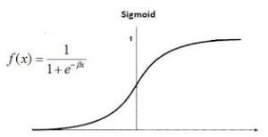
At the core of logistic regression is the logistic (or sigmoid) function, which maps any real valued input to a value between 0 and 1 which is interpreted as a probability. This allows the model to describe the relationship between the input features and the probability of the binary outcome.

Logistic Regression in R Programming

Mathematical Implementation

Logistic regression is a type of **generalized linear model (GLM) used for classification tasks, particularly when the response variable is binary. The goal is to model the probability that a given input belongs to a particular category. The output represents a probability, ranging between 0 and 1. It can we expressed as:

P = \frac{1}{1 + e^{-(\beta_0 + \beta_1 x_1 + \beta_2 x_2 + \cdots + \beta_n x_n)}}

In logistic regression, the **odds represent the ratio of the probability of success to the probability of failure. The **odds ratio (OR) is a key concept that helps interpret logistic regression coefficients. It measures how the odds change with a one-unit increase in a predictor variable:

• An OR of **1 indicates equal probability of success and failure.
• An OR of **2 means success is twice as likely as failure.
• An OR of **0.5 implies failure is twice as likely as success.

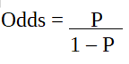
Odd Ratio

Since the outcome is binary and follows a binomial distribution, logistic regression uses the logit link function, which connects the linear model to the probability:

\text{logit}(P) = \log\left( \frac{P}{1 - P} \right) = \beta_0 + \beta_1 x_1 + \beta_2 x_2 + \cdots + \beta_n x_n

This transformation ensures that the predicted probabilities stay within the (0, 1) interval and that the model is linear in the log-odds.

Logistic regression estimates the model parameters using maximum likelihood estimation. This approach finds the coefficients that make the observed outcomes most probable. Each coefficient \beta_i in the logistic regression model represents the change in the log-odds of the outcome for a one-unit increase in the corresponding predictor x_i​, assuming all other variables are held constant.

• If \beta_i > 0, an increase in x_i​ increases the probability of success.
• If \beta_i < 0, an increase in x_i​ decreases the probability of success.

This interpretation is crucial when analyzing how predictor variables influence the predicted outcome.

Code Implementation

We will implement the logistic regression model on he mtcars dataset and make some predictions to see the performance of the model.

1. Importing the Dataset

**mtcars is a built-in dataset in dplyr package in R. We are using the "wt" (weight of the car) and "disp" (displacement of the engine) column as the predictor variable to estimate the engine type. The target variable we are trying to predict is "vs", which tells us whether a car has a V-shaped (0) or straight (1) engine.

R `

install.packages("dplyr") library(dplyr)

head(mtcars)

`

**Output:

Head 0f the Dataset

2. Splitting the Dataset

We are using the caTools package to randomly split the mtcars dataset into two parts: 80% for training (train_reg) and 20% for testing (test_reg). This allows us to train the logistic regression model on one set and evaluate its performance on unseen data.

R `

install.packages("caTools") library(caTools)

split <- sample.split(mtcars, SplitRatio = 0.8)

train_reg <- subset(mtcars, split == "TRUE") test_reg <- subset(mtcars, split == "FALSE")

`

**3. Building the model

Logistic regression is implemented in R using glm() by training the model using features or variables in the dataset.

R `

logistic_model <- glm(vs ~ wt + disp, data = train_reg, family = "binomial") logistic_model

summary(logistic_model)

`

**Output:

Building the model

**In this output:

• **Call: Displays the formula and dataset used for the model.
• **Deviance Residuals: Show how well the model fits the data. Smaller values indicate a better fit.
• **Coefficients: Reflect the impact of each predictor on the outcome. Includes standard errors.
• **Significance Codes: Indicate the statistical significance of each predictor (e.g., ‘***’ means highly significant).
• **Dispersion Parameter: Set to 1 for logistic regression, as it uses a binomial distribution.
• **Null Deviance: The model’s deviance without predictors (only the intercept).
• **Residual Deviance: The model’s deviance after adding predictors. A lower value suggests a better fit.
• **AIC: Used to compare models. Lower AIC indicates a better model with fewer unnecessary variables.
• **Fisher Scoring Iterations: The number of steps taken to find the best-fitting model.

**4. Predict test data based on model

We will use the model to predict some values from out test split****.** For each car in the test set, the model outputs a probability score. A higher score (close to 1) means the model is more confident that the car has a straight engine, while a lower score (close to 0) indicates it's likely a V-shaped engine.

R `

predict_reg <- predict(logistic_model, test_reg, type = "response")

predict_reg <- as.data.frame(predict_reg) predict_reg

`

**Output:

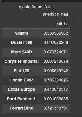
Predict test data based on model

5. Plotting a Confusion Matrix

We are using a confusion matrix to compare actual vs. predicted values, then transforming it into a long format with the melt() function. We create a heatmap with ggplot2 by mapping the counts to tile colors, providing a clear visual of the prediction performance.

R `

library(ggplot2) library(reshape2)

conf_matrix <- table(test_reg$vs, predict_reg)

Reshape the confusion matrix for ggplot2

conf_matrix_melted <- as.data.frame(conf_matrix) colnames(conf_matrix_melted) <- c("Actual", "Predicted", "Count")

ggplot(conf_matrix_melted, aes(x = Actual, y = Predicted, fill = Count)) + geom_tile() + geom_text(aes(label = Count), color = "black", size = 6) + # Add text labels scale_fill_gradient(low = "white", high = "blue") + labs(title = "Confusion Matrix Heatmap", x = "Actual", y = "Predicted") + theme_minimal()

`

**Output:

Confusion Matrix

The confusion matrix shows that the model correctly predicted the negative class (0) 6 times and made 2 false positive errors, predicting 1 when the actual class was 0. It made no false negatives, correctly predicting the positive class (1) once. Overall, the model is performing well, with fewer mistakes in classifying the negative class and no errors in predicting the positive class