Pearson Correlation Testing in R Programming (original) (raw)

Last Updated : 6 Aug, 2025

Pearson correlation is a parametric statistical method used to measure the linear relationship between two continuous variables. It indicates both the strength and direction of the relationship and returns a value between -1 and +1. In R Programming Language it is used to analyze the association between two normally distributed variables.

There are mainly two types of correlation:

1. **Parametric Correlation: It measures a linear dependence between two variables (x and y) is known as a parametric correlation test because it depends on the distribution of the data.
2. **Non-Parametric Correlation: They are rank-based correlation coefficients and are known as non-parametric correlation.

**Pearson Correlation Formula:

\displaystyle r = \frac { \Sigma(x – m_x)(y – m_y) }{\sqrt{\Sigma(x – m_x)^2 \Sigma(y – m_y)^2}}

**Parameters:

• r : pearson correlation coefficient
• x and y: two vectors of length n
• m_x and m_y: corresponds to the means of x and y, respectively.

Implementation of Pearson Correlation Testing

We implement Pearson correlation testing in R using two primary functions:

1. Calculating the Correlation Coefficient Using cor()

We calculate the Pearson correlation coefficient between two numeric vectors using the cor() function.

• **cor: Computes the correlation coefficient between two numeric vectors.
• **x, y: Input numeric vectors of the same length.
• **method: Specifies the correlation method to be used (here, it is "pearson").
• **cat: Used to concatenate and print values. R `

x = c(1, 2, 3, 4, 5, 6, 7) y = c(1, 3, 6, 2, 7, 4, 5) result = cor(x, y, method = "pearson") cat("Pearson correlation coefficient is:", result)

`

**Output:

Pearson correlation coefficient is: 0.5357143

2. Performing Correlation Test Using cor.test()

We perform the Pearson correlation test which returns the coefficient, p-value and confidence interval.

• **cor.test: Performs a test of association between paired samples.
• **t: Test statistic used to calculate the p-value.
• **p-value: Indicates the probability of observing the data under the null hypothesis.
• **alternative hypothesis: States the direction of the correlation (not equal to zero by default).
• **sample estimates: Returns the computed correlation coefficient. R `

x = c(1, 2, 3, 4, 5, 6, 7) y = c(1, 3, 6, 2, 7, 4, 5) result = cor.test(x, y, method = "pearson") print(result)

`

**Output:

Output

In the output above:

• T is the value of the test statistic (T = 1.4186)
• p-value is the significance level of the test statistic (p-value = 0.2152).
• alternative hypothesis is a character string describing the alternative hypothesis (true correlation is not equal to 0).
• sample estimates is the correlation coefficient. For Pearson correlation coefficient it’s named as cor (Cor.coeff = 0.5357).

Implementation for Statistical Significance

We test the statistical significance of correlations using the rcorr function and visualize relationships using ggplot2.

1. Installing and Loading Required Packages

We first install and then load the required packages. We use the built-in mtcars dataset.

• **install.packages: Installs external packages
• **library: Loads the installed packages
• **data: Loads datasets R `

install.packages("ggplot2") install.packages("Hmisc") install.packages("corrplot")

library(ggplot2) library(Hmisc) library(corrplot) data("mtcars")

`

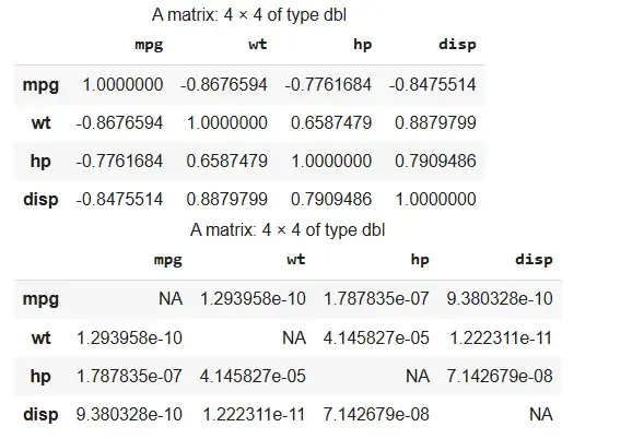
2. Pearson Correlation Testing

We use the rcorr function to calculate Pearson correlation and p-values. It requires data in matrix form.

• **rcorr: Calculates Pearson correlation and significance
• **as.matrix: Converts data frame to matrix
• **cor_test$r: Correlation coefficients
• **cor_test$P: P-values for significance R `

cor_test <- rcorr(as.matrix(mtcars[, c("mpg", "wt", "hp", "disp")]), type = "pearson") cor_test$r cor_test$P

`

**Output:

Output

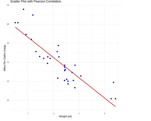
3. Scatter Plot with Regression Line

We use ggplot2 to show the correlation between two variables with a regression line.

• **ggplot: Starts the plot
• **aes: Sets axes
• **geom_point: Plots data points
• **geom_smooth: Adds regression line
• **labs: Adds title and labels
• **theme_minimal: Applies a clean theme R `

ggplot(mtcars, aes(x = wt, y = mpg)) + geom_point(color = "blue", size = 2) + geom_smooth(method = "lm", color = "red", se = FALSE) + labs(title = "Scatter Plot with Pearson Correlation", x = "Weight (wt)", y = "Miles Per Gallon (mpg)") + theme_minimal()

`

**Output:

Output

The scatter plot shows a strong negative correlation between weight and mileage, where heavier cars tend to have lower miles per gallon, as indicated by the downward-sloping red regression line