Plot Probability Distribution Function in R (original) (raw)

Last Updated : 29 Jul, 2025

The PDF is the acronym for Probability Distribution Function and CDF is the acronym for Cumulative Distribution Function. In general, there are many probability distribution functions in R programming Language.

1. PDF

The Probability Density Function (PDF) represents how probability is distributed for a continuous random variable.

**Syntax:

dnorm(x, mean, sd)

**Parameter:

• **x: A numeric vector of values for which the density is to be computed.
• **mean: Mean of the distribution; can be calculated from data or manually assigned.
• **sd: Standard deviation of the distribution; can be calculated from data or manually assigned.

2. CDF

The Cumulative Distribution Function (CDF) gives the probability that a variable takes a value less than or equal to a given number.

**Syntax:

ecdf(x)

**Parameter:

• **x: A numeric vector of values for which the density is to be computed.

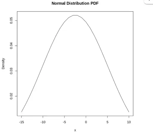
1. Plotting PDF Using plot Function

We generate a normal distribution using dnorm and then plot it using the base R plot function.

• **seq : Generates a sequence of numbers
• **dnorm : Computes the density values of the normal distribution
• **mean : Calculates the average of a numeric vector
• **sd : Calculates the standard deviation of a numeric vector
• **plot : Creates a line plot based on the provided x and y values R `

x <- seq(-15, 10) pdf <- dnorm(x, mean(x), sd(x)) plot(x, pdf, type="l", main="Normal Distribution PDF", xlab="x", ylab="Density")

`

**Output:

Output

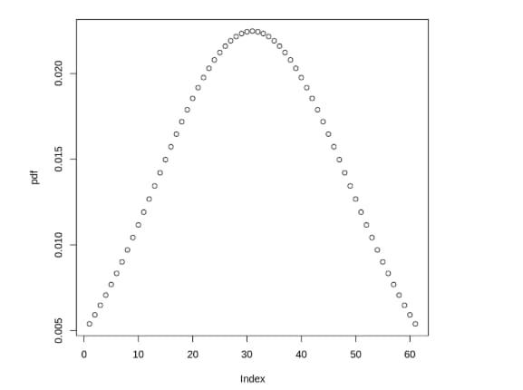
2. Plotting PDF Using plotpdf from gbutils Package

We use plotpdf from the gbutils package to plot the probability distribution curve with quantiles.

• **install.packages : Installs an R package from CRAN
• **library : Loads the installed package for use
• **qnorm : Calculates the quantile values of the normal distribution
• **plotpdf : Plots the given PDF based on quantile range R `

install.packages("gbutils") library(gbutils) x <- seq(-50, 10) pdf <- dnorm(x, mean(x), sd(x)) qdf <- function(x) qnorm(x, mean(x), sd(x)) plotpdf(pdf, qdf, lq = 0.0001, uq = 0.0009)

`

**Output:

Output

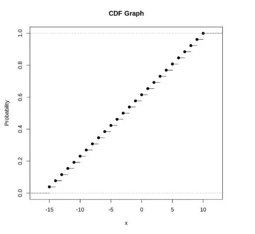
3. Plotting CDF Using plot and ecdf

We compute the cumulative distribution using ecdf and visualize it using plot.

• **ecdf : Computes the empirical cumulative distribution function R `

x <- seq(-15, 10) cdf <- ecdf(x) plot(cdf, main = "CDF Graph", xlab = "x", ylab = "Probability")

`

**Output:

Output

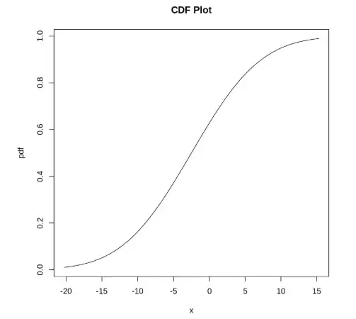
4. Plotting CDF Using plotpdf from gbutils Package

We define a custom cumulative distribution using pnorm and visualize it using plotpdf from the gbutils package.

• **pnorm : Calculates cumulative probability values for the normal distribution R `

install.packages("gbutils") library(gbutils) cdf1 <- function(x) pnorm(x, mean = -2.5, sd = 7.64) plotpdf(cdf1, cdf = cdf1, main = "CDF Plot")

`

**Output:

Output

• The CDF plot shows the cumulative probability increasing from 0 to 1 as the x-values increase.
• It represents the probability that a random variable is less than or equal to a given value.