Regression using kNearest Neighbors in R Programming (original) (raw)
Last Updated : 1 Jul, 2025
The K-Nearest Neighbors (K-NN) is a machine learning algorithm used for both classification and regression tasks. It is a lazy learner algorithm, meaning it doesn’t build an explicit model during training. Instead, it stores the training data and uses it for prediction when new data points need to be classified or predicted.
For regression, K-NN predicts the value of a target variable by averaging the values of its nearest neighbors. This method is based on the idea that similar data points will likely have similar outcomes. In this article, we will focus on using K-NN for regression in R, where we will predict continuous values based on the features of the data points.
Working of K-NN algorithm
The K-Nearest Neighbors (K-NN) algorithm predicts the target value of a new data point by averaging the values of its nearest neighbors. Here's how it works:
- **Select k: Choose the number of neighbors k to consider for prediction. Typically, k is an odd number to avoid ties.
- **Measure Distance: Calculate the distance (often Euclidean) between the new data point and all other points in the dataset. For 2D points (x_1, y_1) and (x_2, y_2), the Euclidean distance is: d = \sqrt{(x_2 - x_1)^2 + (y_2 - y_1)^2}
- **Identify Neighbors: Sort the distances and select the k-nearest neighbors.
- **Predict Outcome: For regression, predict the target value y_{\text{pred}} by averaging the target values of the k-nearest neighbors :y_{\text{pred}} = \frac{1}{k} \sum_{i=1}^{k} y_i
The prediction is based on the average of the neighbors' target values and no explicit model is needed as the algorithm directly uses the training data.
Implementation of K-NN Algorithm for Regression in R
We will not implement the K-NN Algorithm using R programming language and perform regression.
1. Installing Required Packages
To implement K-NN in R, we need the following packages:
- **caTools: For splitting the dataset into training and test sets.
- **class: For the K-NN algorithm.
- **ggplot2: For visualizing the results. R `
install.packages("caTools") install.packages("class") install.packages("ggplot2")
`
2. Loading Libraries and Importing the Dataset
We will load the necessary libraries and import the dataset. For this example, we'll use a dataset that includes customer information such as age, salary and whether or not they purchased a product.
- **read.csv(): Reads the CSV file and imports it into R as a data frame.
- **head(): Displays the first 10 rows of the dataset for a quick look.
You can download the dataset from here : Advertisement.csv
R `
library(caTools) library(class) library(ggplot2)
dataset = read.csv('Advertisement.csv') head(dataset)
`
**Output:
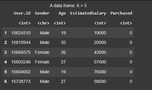
Dataset
3. Preprocessing the Data
Before applying K-NN, we need to encode the target variable (Purchased) as a factor and split the dataset into training and testing sets.
- **factor(): Converts the target variable (Purchased) to a factor, ensuring it’s treated as categorical.
- **sample.split(): Splits the dataset into a training set (75%) and a test set (25%).
- **scale(): Standardizes the feature columns by subtracting the mean and dividing by the standard deviation. R `
set.seed(123) split = sample.split(dataset$Purchased, SplitRatio = 0.75) training_set = subset(dataset, split == TRUE) test_set = subset(dataset, split == FALSE)
training_set[, c(3, 4)] = scale(training_set[, c(3, 4)]) test_set[, c(3, 4)] = scale(test_set[, c(3, 4)])
`
4. Applying K-NN for Regression
We will now apply the K-NN algorithm to the training set and predict the outcomes for the test set. We will use knn() function to implements the K-NN algorithm.
- **train: The feature columns from the training set.
- **test: The feature columns from the test set.
- **cl: The target variable (Purchased) from the training set.
- **k = 5: The number of neighbors to consider for prediction.
- **prob = TRUE: Provides the probability of the predicted outcome. R `
y_pred = knn(train = training_set[,c(3,4)], test = test_set[, c(3,4)], cl = training_set[, 5], k = 5, prob = TRUE)
`
5. Evaluating the Model
We will create a confusion matrix to evaluate how well the model performs on the test set.
- **cm = table(test_set[, 5], y_pred): Creates a confusion matrix comparing actual vs predicted values.
- **cm_df <- as.data.frame(cm): Converts the confusion matrix into a data frame.
- **colnames(cm_df) <- c("Actual", "Predicted", "Count"): Renames columns for clarity.
- **ggplot(cm_df, aes(x = Actual, y = Predicted, fill = Count)): Sets up the plot with Actual on the x-axis, Predicted on the y-axis and Count for tile color.
- **geom_tile(): Creates heatmap tiles based on the fill aesthetic.
- **geom_text(aes(label = Count), color = "white", size = 5): Adds text labels (count values) inside the tiles. R `
cm = table(test_set[, 5], y_pred)
cm_df <- as.data.frame(cm) colnames(cm_df) <- c("Actual", "Predicted", "Count")
ggplot(cm_df, aes(x = Actual, y = Predicted, fill = Count)) + geom_tile() + geom_text(aes(label = Count), color = "white", size = 5) + scale_fill_gradient(low = "lightblue", high = "steelblue") + theme_minimal() + labs(title = "Confusion Matrix Heatmap", x = "Predicted", y = "Actual") + theme(axis.text.x = element_text(angle = 45, hjust = 1))
`
**Output:
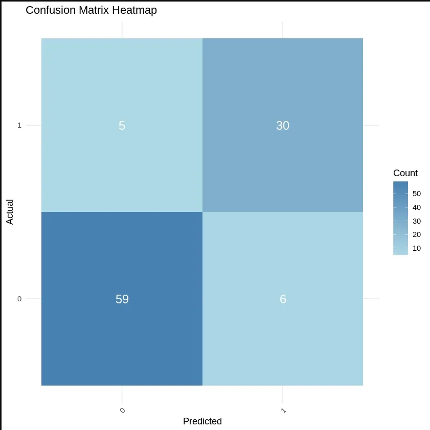
Evaluating the Model
6. Visualizing the Results
We will visualize the results using a plot to show how well the model has fit the training and test data.
- **ggplot(data = grid_set, aes(x = Age, y = EstimatedSalary, color = factor(y_grid))): Initializes a plot using the grid data and assigns color based on the predicted outcome from K-NN.
- **geom_tile(aes(fill = factor(y_grid)), alpha = 0.3): Adds tiles to the plot with colors based on the predicted outcome (**y_grid), setting transparency to 0.3.
- **geom_point(data = set1, aes(x = Age, y = EstimatedSalary, color = factor(Purchased))): Adds actual data points from the training set, coloring by the true Purchased value.
**6.1. Training Set: We will visualize the decision boundary of the model using ggplot2 library.
- **set1 = training_set: Creates a copy of the training dataset for reference in visualization.
- **X1 = seq(min(set[, 3]) - 1, max(set[, 3]) + 1, by = 0.01): Generates a sequence of values for Age (column 3) with a small buffer (1) to cover the range.
- **X2 = seq(min(set[, 4]) - 1, max(set[, 4]) + 1, by = 0.01): Generates a sequence of values for Estimated Salary (column 4) with a small buffer.
- **labs(title = "K-NN Classification (Training Set)", x = "Age", y = "Estimated Salary"): Adds a title and labels to the axes.
- **grid_set = expand.grid(X1, X2): Creates a grid of all combinations of Age and Estimated Salary values.
- **y_grid = knn(train = training_set[, 3:4], test = grid_set, cl = training_set[, 5], k = 5): Applies the K-NN algorithm to predict the target (Purchased) based on the grid of Age and Estimated Salary. R `
set1 = training_set
X1 = seq(min(set[, 3]) - 1, max(set[, 3]) + 1, by = 0.01) X2 = seq(min(set[, 4]) - 1, max(set[, 4]) + 1, by = 0.01) grid_set = expand.grid(X1, X2)
colnames(grid_set) = c('Age', 'EstimatedSalary')
y_grid = knn(train = training_set[, 3:4], test = grid_set, cl = training_set[, 5], k = 5)
ggplot(data = grid_set, aes(x = Age, y = EstimatedSalary, color = factor(y_grid))) + geom_tile(aes(fill = factor(y_grid)), alpha = 0.3) + geom_point(data = set1, aes(x = Age, y = EstimatedSalary, color = factor(Purchased))) + labs(title = "K-NN Classification (Training Set)", x = "Age", y = "Estimated Salary") + scale_fill_manual(values = c("tomato", "springgreen3")) + scale_color_manual(values = c("red3", "green4"))
`
Output:
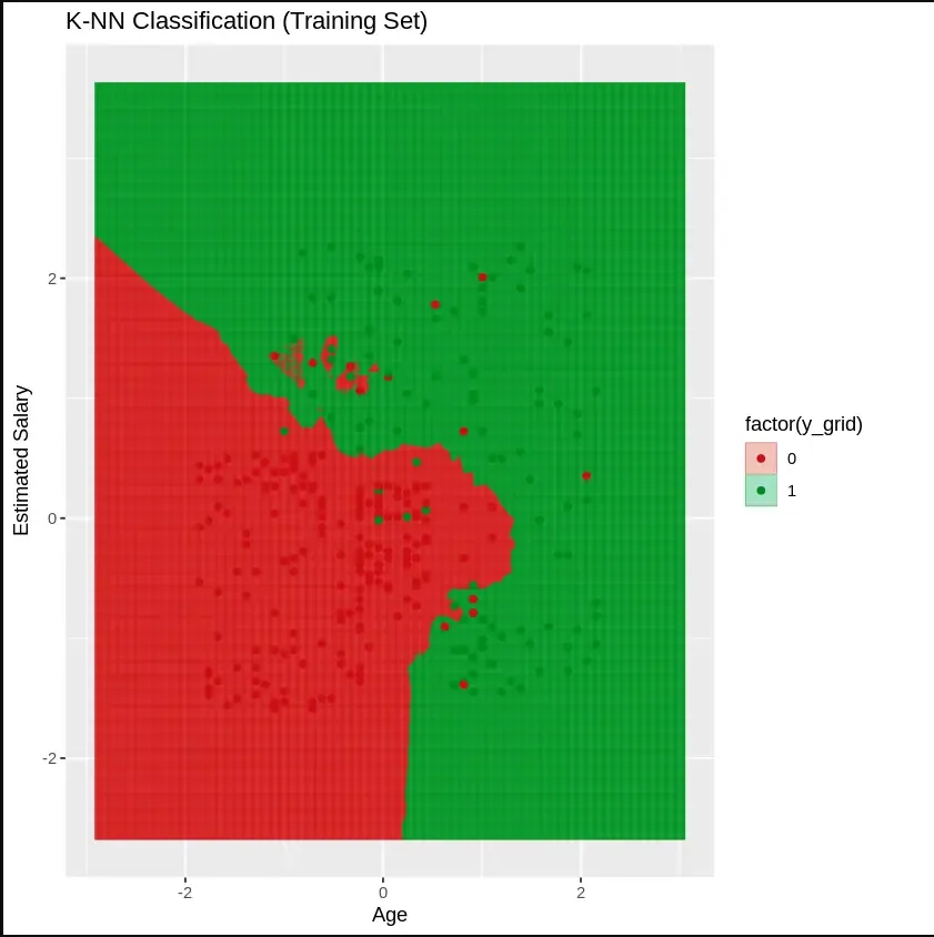
Training Set
**6.2. Testing Set: We will visualize the decision boundary of the model using ggplot2 library.
- **set2 = test_set: Creates a reference to the test dataset for visualization.
- **X1 = seq(min(set[, 3]) - 1, max(set[, 3]) + 1, by = 0.01): Generates a sequence of values for Age (column 3) in the test set, with a small buffer to cover the range.
- **X2 = seq(min(set[, 4]) - 1, max(set[, 4]) + 1, by = 0.01): Generates a sequence of values for Estimated Salary (column 4) in the test set.
- **grid_set = expand.grid(X1, X2): Creates a grid of all combinations of Age and Estimated Salary values. R `
set2 = test_set
X1 = seq(min(set[, 3]) - 1, max(set[, 3]) + 1, by = 0.01) X2 = seq(min(set[, 4]) - 1, max(set[, 4]) + 1, by = 0.01) grid_set = expand.grid(X1, X2)
colnames(grid_set) = c('Age', 'EstimatedSalary')
y_grid = knn(train = training_set[, 3:4], test = grid_set, cl = training_set[, 5], k = 5)
ggplot(data = grid_set, aes(x = Age, y = EstimatedSalary, color = factor(y_grid))) + geom_tile(aes(fill = factor(y_grid)), alpha = 0.3) + geom_point(data = set2, aes(x = Age, y = EstimatedSalary, color = factor(Purchased))) + labs(title = "K-NN Classification (Test Set)", x = "Age", y = "Estimated Salary") + scale_fill_manual(values = c("tomato", "springgreen3")) + scale_color_manual(values = c("red3", "green4"))
`
**Output:
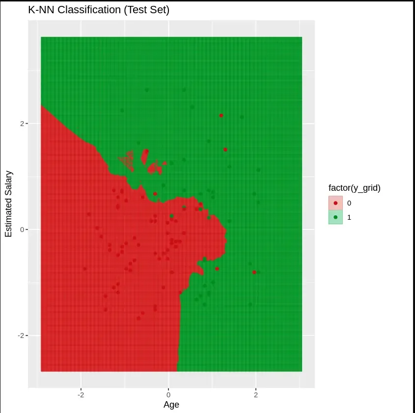
Testing Set:
Advantages of K-Nearest Neighbors (K-NN)
- **No Training Period: K-NN is an instance-based learning algorithm, meaning it doesn’t require a training phase.
- **Adaptability: New data can be added seamlessly without retraining the model.
- **Simple Implementation: K-NN is easy to understand and implement, with only two key parameters: k and the distance function.
Disadvantages of K-Nearest Neighbors (K-NN)
- **Computational Cost: K-NN can be slow for large datasets because it calculates the distance to every data point.
- **High Dimensionality: The algorithm struggles with high-dimensional data, where the number of features is large.
- **Sensitive to Noise: K-NN is sensitive to noisy or irrelevant features, which can impact the model's accuracy.