Visualize Confusion Matrix Using Caret Package in R (original) (raw)

Last Updated : 3 May, 2025

The Confusion Matrix is a type of matrix that is used to visualize the predicted values against the actual Values. The row headers in the confusion matrix represent predicted values and column headers are used to represent actual values. The Confusion matrix contains four cells as shown in the below image.

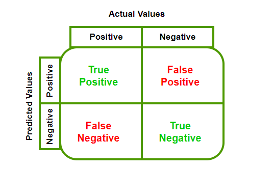
Visualize Confusion Matrix Using Caret Package in R

Confusion Matrix

**True Negative (TN): Negative values predicted correctly as negative.
**False Positive (FP): Negative values predicted wrongly as positive.
**False Negative (FN): Positive values predicted wrongly as negative.
**True Positive (TP): Positive values predicted correctly as positive

ConfusionMatrix() function

In R Programming the Confusion Matrix can be visualized using confusionMatrix() function which is present in the caret package.

**Syntax

confusionMatrix(data, reference, positive = NULL, dnn = c("Prediction", "Reference"))

where

**data:a factor of predicted classes.
**reference: a factor of classes to be used as the true results.
**positive(optional): an optional character string for the factor level.
**dnn(optional): a character vector of dimnames for the table.

Step to Create Confusion Matrix

**Step 1: Install and load the caret package.

R `

install.packages("caret") library(caret)

**Step 2: Define predicted and actual values.

R `

pred_values <- factor(c(TRUE, FALSE, FALSE, TRUE, FALSE, TRUE, FALSE)) actual_values <- factor(c(FALSE, FALSE, TRUE, TRUE, FALSE, TRUE, TRUE))

**Step 3: Generate the confusion matrix.

R `

cf <- caret::confusionMatrix(data=pred_values, reference=actual_values) print(cf)

**Output:

Confusion Matrix and Statistics
Reference
Prediction FALSE TRUE
FALSE 2 2
TRUE 1 2

Accuracy : 0.5714
95% CI : (0.1841, 0.901)
No Information Rate : 0.5714
P-Value [Acc > NIR] : 0.6531

Kappa : 0.16
Mcnemar's Test P-Value : 1.0000

Sensitivity : 0.6667
Specificity : 0.5000
Pos Pred Value : 0.5000
Neg Pred Value : 0.6667
Prevalence : 0.4286
Detection Rate : 0.2857
Detection Prevalence : 0.5714
Balanced Accuracy : 0.5833
'Positive' Class : FALSE

The confusion matrix gives us detailed statistics, including accuracy, sensitivity, specificity, and Kappa.

Visualizing Confusion Matrix

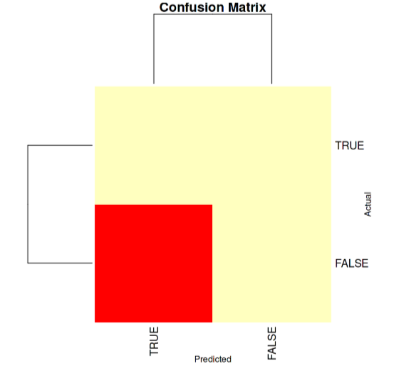
**using fourfoldplot() function: The fourfoldplot() function can visually represent the confusion matrix. To use it, we need to convert the confusion matrix into a table format.

R `

fourfoldplot(as.table(cf),color=c("yellow","pink"),main = "Confusion Matrix")

**Output:

confusion_matrix

Visualize Confusion Matrix Using Caret Package in R

**Using Heatmap: Another approach is to visualize the confusion matrix using a heatmap

R `

conf_matrix <- table(actual, predicted)

Visualize the confusion matrix using heatmap

heatmap(conf_matrix, main = "Confusion Matrix", xlab = "Predicted", ylab = "Actual", col = heat.colors(10), scale = "column", margins = c(5, 5))

**Output:

confusion_matrix_2

Visualize Confusion Matrix

In this example, the table() function is used to create the confusion matrix directly. The heatmap() function then visualizes the matrix.

Measuring the performance

We will Measuring the performance of our model using accuracy and using this formula.

Accuracy = (TP + FP) / Total Observations

Confusion Matrix with gmodels Package

To create a confusion matrix using the "gmodels" package in R, we use the CrossTable() function. This function allows us to create a cross-tabulation table, which is essentially a confusion matrix.

R `

library(gmodels)

Example data (actual and predicted classes)

actual_values <- c("Positive", "Negative", "Positive", "Negative", "Positive", "Positive") pred_values <- c("Positive", "Negative", "Positive", "Negative", "Negative", "Positive")

Create a confusion matrix using CrossTable

confusion_matrix <- CrossTable(actual_values, pred_values, prop.chisq = FALSE, prop.t = FALSE, prop.r = FALSE)

Print the confusion matrix

print(confusion_matrix)

**Output:

Cell Contents
|-------------------------|
| N |

N / Col Total

Total Observations in Table: 6

          | pred_values

actual_values	Negative	Positive	Row Total

 Negative |         2 |         0 |         2 |   
          |     0.667 |     0.000 |           |

--------------|-----------|-----------|-----------|
Positive | 1 | 3 | 4 |
| 0.333 | 1.000 | |

--------------|-----------|-----------|-----------|
Column Total | 3 | 3 | 6 |
| 0.500 | 0.500 | |

--------------|-----------|-----------|-----------|

$t
y
x Negative Positive
Negative 2 0
Positive 1 3

$prop.row
y
x Negative Positive
Negative 1.00 0.00
Positive 0.25 0.75

$prop.col
y
x Negative Positive
Negative 0.6666667 0.0000000
Positive 0.3333333 1.0000000

$prop.tbl
y
x Negative Positive
Negative 0.3333333 0.0000000
Positive 0.1666667 0.5000000

In classification problems, "actual" is used to denote the true labels and "predicted" to denote the predictions of the model. A confusion matrix is used to compare predicted labels to actual ones in order to measure model performance. The CrossTable() command from the "gmodels" package in R creates such a matrix. Proportions (accuracy, precision, recall, etc.) are disabled by default by setting prop.chisq, prop.t, and prop.r to FALSE.