mlr3 Package in R (original) (raw)

Last Updated : 23 Jul, 2025

The mlr3 package is a modern machine learning framework for R that simplifies building, evaluating and tuning machine learning models. It provides a unified interface for various machine learning tasks, such as classification, regression and clustering, allowing users to focus on creating models rather than handling complex workflows.

Key Features of mlr3

**Unified Interface: A consistent API for various machine learning algorithms and tasks, simplifying experimentation.
**Task and Learner System: Separates tasks (problems) and learners (models), making it easy to switch algorithms.
**Performance Evaluation: Built-in metrics like accuracy, precision and recall for evaluating models.
**Resampling and Cross-Validation: Flexible methods like k-fold and bootstrapping for model evaluation.
**Hyperparameter Tuning: Optimizes model performance with automatic hyperparameter tuning.
**Parallelization: Accelerates training and evaluation for large datasets and complex models.
**Extensibility: Easily add new learners, tasks and metrics to suit our needs.

Implementation of SVM Classifier using mlr3

We will implement a machine learning model using the mlr3 package with Support Vector Machine (SVM). We will use the iris dataset and build a classification model using an SVM.

1. Installing and Loading Required Packages

Before starting, we need to install and load the mlr3, e1071 and mlr3learners packages. The mlr3learners package provides a set of common learners but to use SVM we need e1071 library.

**install.packages(): Installs the required packages.
**library(): Loads the package so we can use its functions. R `

install.packages("mlr3") install.packages("mlr3learners")

library(mlr3) library(mlr3learners)

2. Loading the Dataset

We will use the built-in iris dataset in R which contains 150 observations of iris flowers, with 4 features: Sepal.Length, Sepal.Width, Petal.Length and Petal.Width. The target variable is the species of the flower.

R `

data("iris") head(iris)

**Output:

data

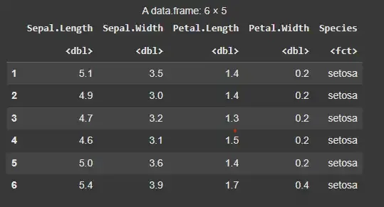
Loading the Dataset

3. Creating the Task

In mlr3, a task represents the machine learning problem. We create a classification task where the target variable is the species of the flowers.

**id: A unique identifier for the task.
**backend: The dataset to be used for the task (in this case, the iris dataset).
**target: The column that contains the target variable (Species in this case). R `

task <- TaskClassif$new(id = "iris", backend = iris, target = "Species")

4. Creating the Learner

A learner represents a machine learning algorithm. Here, we will use the Support Vector Machine (SVM) algorithm, which is available through the e1071 package.

**classif.svm: The learner name representing the Support Vector Machine (SVM) algorithm for classification. R `

learner <- lrn("classif.svm")

5. Training the Model

Now, we can train the SVM model using the train method. The learner is trained on the task created earlier.

**train(): Trains the model on the provided task. R `

learner <- lrn("classif.svm")

6. Making Predictions

After training the model, we can use it to make predictions. The predict method is used to make predictions on the task (either on the training data or a test set).

**predict(): Generates predictions from the trained model. R `

predictions <- learner$predict(task)

print(predictions)

**Output:

clf

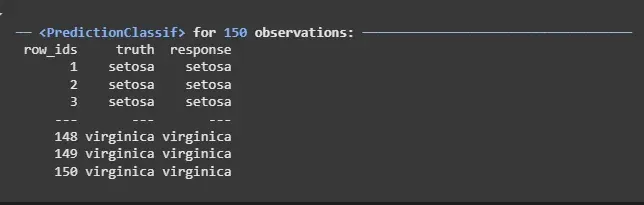
Making Predictions

7. Evaluating the Model

We evaluate the model’s performance using a performance measure like accuracy. The score() method is used to calculate the accuracy of the predictions.

**score(): Evaluates the model’s performance using a specified metric (e.g., accuracy). R `

accuracy <- predictions$score(msr("classif.acc")) print(accuracy)

**Output:

classif.acc
0.9733333

8. Visualizing the Decision Boundary

To visualize the SVM model, we can plot the decision boundary and support vectors. We'll use only two features (Sepal.Length and Sepal.Width) for simplicity.

**ggplot(): Used for creating a plot with custom layers.
**geom_point(): Adds points to the plot (for data points).
**geom_abline(): Adds a line (for decision boundary).
**geom_vline(), geom_hline(): Add vertical and horizontal lines for support vectors. R `

svm_model <- learner$train(task)

xrange <- seq(from = min(iris$Sepal.Length), to = max(iris$Sepal.Length), length.out = 100) yrange <- seq(from = min(iris$Sepal.Width), to = max(iris$Sepal.Width), length.out = 100)

grid <- expand.grid(Sepal.Length = xrange, Sepal.Width = yrange)

grid_predictions <- predict(learner, newdata = grid)

ggplot(iris, aes(x = Sepal.Length, y = Sepal.Width, color = Species)) + geom_point(alpha = 0.7) + geom_point(data = grid, aes(x = Sepal.Length, y = Sepal.Width, color = as.factor(grid_predictions$score)), shape = 1, alpha = 0.3) + theme_minimal() + labs(title = "SVM Decision Boundary (Sepal.Length vs Sepal.Width)", x = "Sepal Length", y = "Sepal Width")

**Output:

decision-

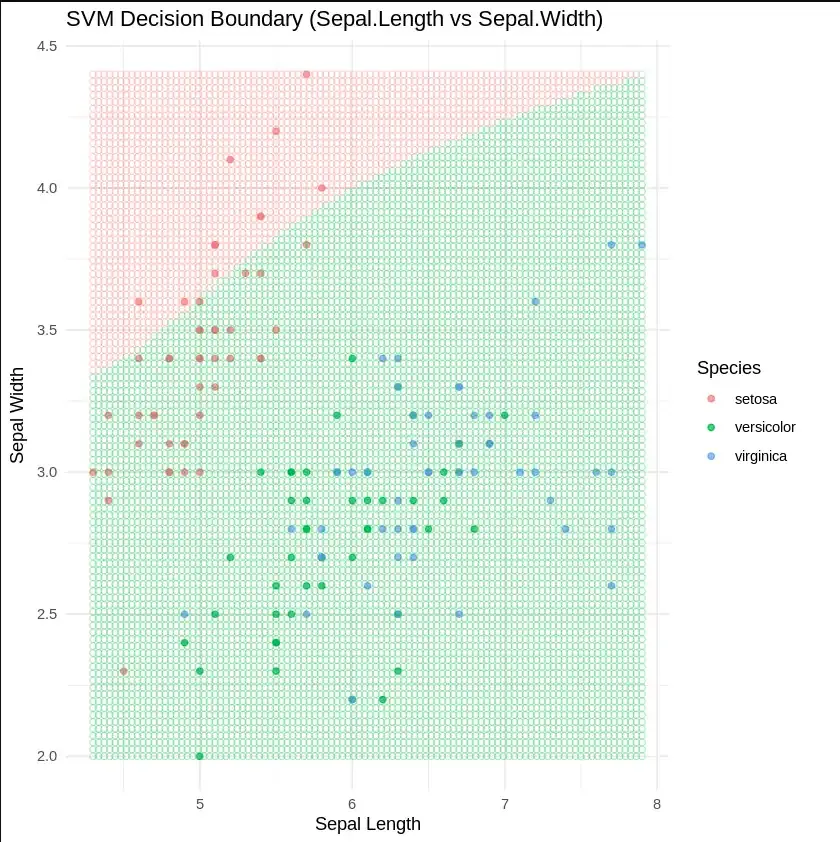
Visualizing the Decision Boundary

9. 3-Dimensional Visualization Using Plotly

To better visualize the decision boundaries we will use ploty to create a 3D plot of our model. Since it will be better to render a HTML file , we will export our plot into a HTML file for better viewing.

**plot_ly(): Initializes an empty Plotly figure to build the plot.
**add_markers(): Adds markers to the plot for the grid points and the original iris dataset, with colors representing the predicted classes.
**layout(): Configures the plot layout, including titles for the plot and axis labels for Sepal Length, Sepal Width and Petal Length.
**saveWidget(): Saves the plot as an interactive HTML file, making it viewable in a web browser.
**system(): Executes system commands to move the HTML file and associated assets to a specific directory and zip them for download. R `

install.packages("plotly") install.packages("htmlwidgets")

library(plotly) library(htmlwidgets)

x_seq <- seq(min(iris$Sepal.Length), max(iris$Sepal.Length), length.out = 20) y_seq <- seq(min(iris$Sepal.Width), max(iris$Sepal.Width), length.out = 20) z_seq <- seq(min(iris$Petal.Length), max(iris$Petal.Length), length.out = 20)

grid <- expand.grid( Sepal.Length = x_seq, Sepal.Width = y_seq, Petal.Length = z_seq )

grid$Petal.Width <- mean(iris$Petal.Width)

grid_preds <- learner$predict_newdata(grid) grid$Predicted <- grid_preds$response

colors <- c("setosa" = "red", "versicolor" = "green", "virginica" = "blue") iris$Color <- colors[iris$Predicted] grid$Color <- colors[grid$Predicted]

fig <- plot_ly()

fig <- fig %>% add_markers( data = grid, x = ~Sepal.Length, y = ~Sepal.Width, z = ~Petal.Length, color = ~Predicted, colors = colors, marker = list(size = 2, opacity = 0.2), showlegend = FALSE )

fig <- fig %>% add_markers( data = iris, x = ~Sepal.Length, y = ~Sepal.Width, z = ~Petal.Length, color = ~Predicted, colors = colors, marker = list(size = 6), name = "Iris Points" ) %>% layout( title = "SVM 3D Classification (Plotly)", scene = list( xaxis = list(title = "Sepal Length"), yaxis = list(title = "Sepal Width"), zaxis = list(title = "Petal Length") ) )

saveWidget(fig, "svm_plotly_3d.html", selfcontained = FALSE)

system("mv svm_plotly_3d.html /content/") system("mv svm_plotly_3d_files /content/") system("zip -r /content/svm_plotly.zip /content/svm_plotly_3d.html /content/svm_plotly_3d_files")

cat("Download files: svm_plotly.zip)")

**Output:

plo

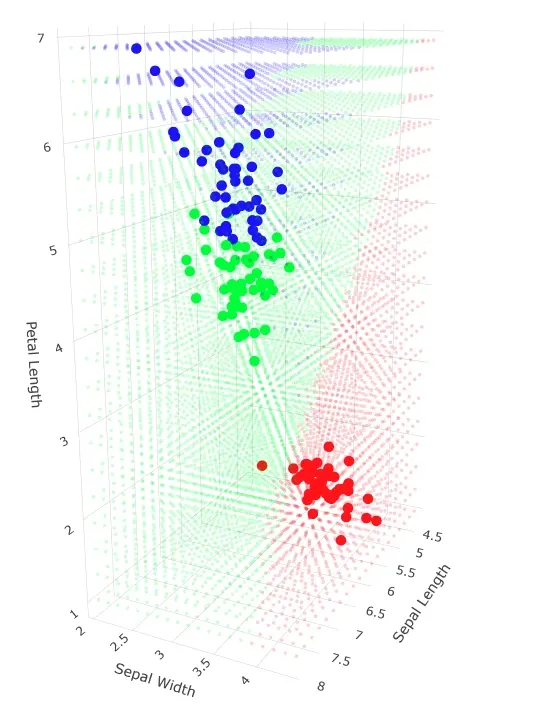
3D plot showing Decision Boundary

svmp1

3-Dimensional Visualization

Advantages of mlr3

There several advantages when using mlr3 package for machine learning:

**Simplicity and Flexibility: mlr3 streamlines the process of training, evaluating and tuning machine learning models while providing us with the flexibility to customize the workflow according to our needs.
**Extensibility: We can easily extend the framework by incorporating custom learners, tasks, or measures to suit our specific requirements.
**Robust Evaluation: With built-in support for cross-validation, resampling and hyperparameter tuning, we can efficiently assess model performance and ensure its robustness.
**Parallelism: mlr3 enables parallel processing, allowing us to scale model training and evaluation to handle large datasets more efficiently.

In this article, we explored the mlr3 package in R, which provides a comprehensive and flexible framework for machine learning. We also demonstrated how to build an SVM model, evaluate its performance and tune its hyperparameters.