Netflix Stock Price Prediction & Forecasting using Machine Learning in R (original) (raw)

Last Updated : 23 Jun, 2025

In simple words, "Stock" is the ownership of a small part of a company. The more stock you have the bigger the ownership is. Stock price prediction is challenging due to the dynamic and volatile nature of stock prices. We will be using machine learning algorithms to predict a company's stock price aims to forecast the future value of the company stock.

Project Overview

We will predict Netflix Stock Prices using machine learning algorithms in R. We will use the ARIMA model to predict the future stock prices of Netflix based on historical data.

Understanding our Dataset

For this project, we use Netflix's historical stock price data from 2002-01-01 to 2022-12-31. The dataset contains the following columns:

**NFLX.Open: The opening price of Netflix stock for a given day.
**NFLX.High: The highest price of Netflix stock on that day.
**NFLX.Low: The lowest price of Netflix stock on that day.
**NFLX.Close: The closing price of Netflix stock on that day.
**NFLX.Volume: The volume of stocks traded on that day.
**NFLX.Adjusted: The adjusted closing price after splits and dividends.

We focus on the **NFLX.Close column for stock price prediction.

You can download the dataset from here: NFLX.csv

1. Importing Required Libraries

We start by installing and loading the necessary libraries for time series analysis and forecasting.

**forecast: Used for modeling and forecasting time series data.
**quantmod: Helps fetch financial market data.
**tseries: Provides functions for time series analysis.
**ggplot2: Support visualization and handle missing data. R `

install.packages(c("forecast", "xts","tseries","ggplot2")) library(forecast) library(xts) library(tseries) library(ggplot2)

2. Loading the Netflix Stock Price Dataset

We load the Netflix stock price data either from a CSV file and print the first few rows (head(df)) to verify the data structure.

R `

df = read.csv("/content/NFLX.csv") head(df)

**Output:

data

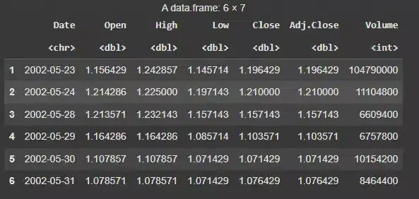
Netflix Stock Price Dataset

3. Checking the Dataset

We will check the dataset's dimensions and identify any missing values to ensure the data is clean for modeling.

R `

dim(df) print(colSums(is.na(df)))

**Output:

null

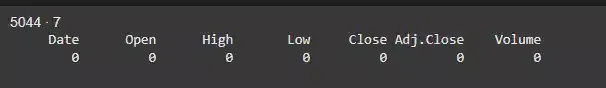
Netflix Stock Price Prediction & Forecasting using Machine Learning in R

The dataset has 5044 rows and 7 columns and there are no missing values in the dataset. By checking for missing values we ensure that we don't have any incomplete data, which could affect model accuracy.

4. Getting the Summary of the Data

We take a summary of the data to get an overview of the stock's behavior, such as minimum, maximum and average values.

R `

summary(df)

**Output:

summary

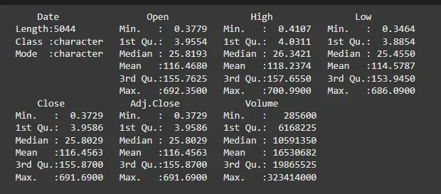
Summary of the Data

The summary provides a overview of the distribution of stock prices. The mean and median help identify the average stock price, while the max and min give us the extremes of the dataset. These values show that Netflix’s stock price has fluctuated significantly over time.

5. Plotting the Data

We visualize the stock price data using the chartSeries() function from the quantmod package to observe the trends in stock prices.

**df[, -1]: Removes the first column (which is assumed to be the date column).
**as.Date(df[, 1]): Converts the first column (the date column) into a Date format.
**xts(): Converts the data frame into an xts object, which is required by chartSeries(). R `

df.xts <- xts(df[, -1], order.by = as.Date(df[, 1]))

chartSeries(df.xts, type = 'auto')

**Output:

chart

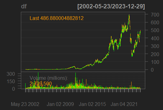
Plotting the Data

The **chartSeries() function automatically generates a suitable chart (candlestick or line chart) for the stock price, which visually displays trends, patterns and fluctuations in Netflix’s stock price over time.

6. Checking for Stationarity

We check if the data is stationary using visualizations. Non-stationary data needs to be transformed before forecasting.

R `

ggplot(df, aes(x = Close)) + geom_density(alpha = 0.5, fill = "blue") + geom_histogram(aes(y = ..density..), color = "black", fill = "lightgray", bins = 30, alpha = 0.4) + labs(title = "Density and Histogram of Close Price", x = "Close Price", y = "Density") + theme_minimal()

**Output:

stationary

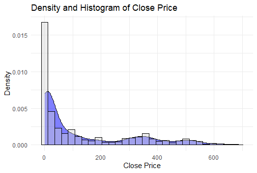
Checking for Stationarity

The histogram and density plot show that the data is non-stationary, as it is not normally distributed and shows a trend.

**Note: A stationary time series has a constant mean, variance and autocorrelation over time. The non-stationary nature of the data indicates that it has trends and needs to be differenced or transformed before applying the ARIMA model.

7. Splitting our Dataset

We separate the Close price (the target variable) into training and testing datasets. The data is split into training and testing sets (80:20 ratio). The training set will be used to fit the model, while the testing set will validate the model's performance.

R `

df.close = df[,4] df.close.train = df.close[1:(0.8 * length(df.close))] df.close.test = df.close[(0.8 * length(df.close)):length(df.close)]

8. Fitting the Model

We use the ARIMA model for forecasting. The **auto.arima() function automatically selects the best ARIMA model by testing various combinations of the parameters.

**p: Number of AR (AutoRegressive) terms (lags of the series).
****d:**Number of differencing operations needed to make the series stationary.
**q: Number of MA (Moving Average) terms (lags of the forecast errors). R `

df.close.arima = auto.arima(df.close.train, seasonal = TRUE, stepwise = TRUE, nmodels = 100, trace = TRUE, biasadj = TRUE) summary(df.close.arima)

**Output:

model_summ

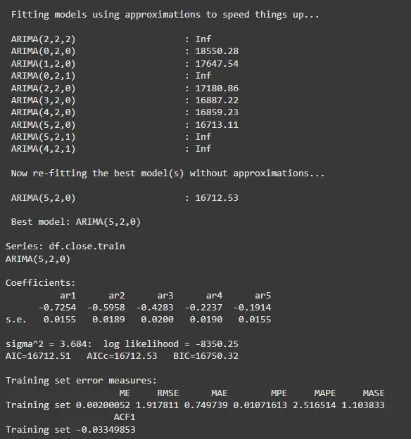
Fitting the Model

9. Evaluating the Model

We check the model's performance by comparing the forecast results on the training and test data.

R `

accuracy(df.close.forecast, df.close.test)

**Output:

acc

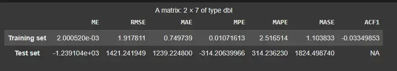
Evaluating the Model

The training set has minimal errors across all metrics (ME, RMSE, MAE), suggesting the model fits well on the training data. However, the test set shows higher errors, indicating the model's poor generalization to unseen data (potential overfitting).

10. Predicting Netflix Stock Prices

Finally, we predict the stock prices using our ARIMA model for the next 7 days, visualize the predicted stock prices and compare them with the actual test data to evaluate the model's performance.

R `

pred1 = predict(df.close.arima, n.ahead = 7)

forecasted_values = pred1$pred

forecast_dates = seq(from = as.Date("2022-06-03"), by = "days", length.out = 7) forecast_df = data.frame(Date = forecast_dates, Predicted = forecasted_values)

ggplot(forecast_df, aes(x = Date, y = Predicted)) + geom_line(color = "blue") +
geom_point(color = "red") + labs(title = "Predicted Netflix Stock Prices for Next 30 Days", x = "Date", y = "Predicted Stock Price") + theme_minimal()

**Output:

forecast

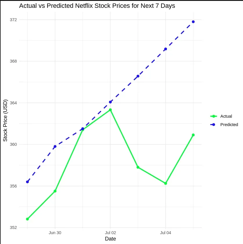
Predicting Netflix Stock Prices

Conclusion

From our analysis, we concluded that predicting Netflix stock prices using the ARIMA model can provide reasonable forecasts. However, the model showed signs of overfitting, as it performed well on the training set but not on new, unseen data. This suggests that improvements such as parameter tuning or using more sophisticated models could help enhance the prediction accuracy for stock prices.