rand vs normal in Numpy.random in Python (original) (raw)

Last Updated : 17 Nov, 2020

In this article, we will look into the principal difference between the Numpy.random.rand() method and the Numpy.random.normal() method in detail.

• About random: For random we are taking .rand()
  numpy.random.rand(d0, d1, …, dn) :
  creates an array of specified shape and
  fills it with random values.
  Parameters :
  d0, d1, ..., dn : [int, optional]
  Dimension of the returned array we require,
  If no argument is given a single Python float
  is returned.
  Return :
  Array of defined shape, filled with random values.
• About normal: For random we are taking .normal()
  numpy.random.normal(loc = 0.0, scale = 1.0, size = None) : creates an array of specified shape and fills it with random values which is actually a part of Normal(Gaussian)Distribution. This is Distribution is also known as Bell Curve because of its characteristics shape.
  Parameters :
  loc : [float or array_like]Mean of
  the distribution.
  scale : [float or array_like]Standard
  Derivation of the distribution.
  size : [int or int tuples].
  Output shape given as (m, n, k) then
  mnk samples are drawn. If size is
  None(by default), then a single value
  is returned.
  Return :
  Array of defined shape, filled with
  random values following normal
  distribution.

Code 1 : Randomly constructing 1D array

Output :

1D Array filled with random values : [ 0.84503968 0.61570994 0.7619945 0.34994803 0.40113761]

Code 2 : Randomly constructing 1D array following Gaussian Distribution

import numpy as geek

array = geek.random.normal( 0.0 , 1.0 , 5 )

print ( "1D Array filled with random values "

`` "as per gaussian distribution : \n" , array)

array = geek.random.normal( 0.0 , 1.0 , ( 2 , 1 , 2 ))

print ( "\n\n3D Array filled with random values "

`` "as per gaussian distribution : \n" , array)

Output :

1D Array filled with random values as per gaussian distribution : [-0.99013172 -1.52521808 0.37955684 0.57859283 1.34336863]

3D Array filled with random values as per gaussian distribution : [[[-0.0320374 2.14977849]]

[[ 0.3789585 0.17692125]]]

Code3 : Python Program illustrating graphical representation of random vs normal in NumPy

import numpy as geek

import matplotlib.pyplot as plot

mean = 0

std = 0.1

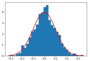
array = geek.random.normal( 0 , 0.1 , 1000 )

print ( "1D Array filled with random values "

`` "as per gaussian distribution : \n" , array);

count, bins, ignored = plot.hist(array, 30 , normed = True )

plot.plot(bins, 1 / (std * geek.sqrt( 2 * geek.pi)) *

`` geek.exp( - (bins - mean) * * 2 / ( 2 * std * * 2 ) ),

`` linewidth = 2 , color = 'r' )

plot.show()

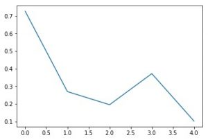
random_array = geek.random.rand( 5 )

print ( "1D Array filled with random values : \n" , random_array)

plot.plot(random_array)

plot.show()

Output :

1D Array filled with random values as per gaussian distribution : [ 0.12413355 0.01868444 0.08841698 ..., -0.01523021 -0.14621625 -0.09157214]

1D Array filled with random values : [ 0.72654409 0.26955422 0.19500427 0.37178803 0.10196284]

Important :
In code 3, plot 1 clearly shows Gaussian Distribution as it is being created from the values generated through random.normal() method thus following Gaussian Distribution.
plot 2 doesn’t follow any distribution as it is being created from random values generated by random.rand() method.

Note :
Code 3 won’t run on online-ID. Please run them on your systems to explore the working.
.