Simple Linear Regression in Python (original) (raw)
Last Updated : 16 Jan, 2025
Simple linear regression models the relationship between a dependent variable and a single independent variable. In this article, we will explore simple linear regression and it's implementation in Python using libraries such as NumPy, Pandas, and scikit-learn.
Understanding Simple Linear Regression
**Simple Linear Regression aims to describe how one variable i.e the dependent variable changes in relation with reference to the independent variable. For example consider a scenario where a company wants to predict sales based on advertising expenditure. By using simple linear regression the company can determine if an increase in advertising leads to higher sales or not.
The below graph explains the relationship between advertising expenditure and sales using simple linear regression:

Simple Linear Regression
The relationship between the dependent and independent variables is represented by the simple linear equation:
y=mx+b
Here:
- y is the predicted value (dependent variable).
- m is the slope of the line
- x is the independent variable.
- b is the y-intercept (the value of y when x is 0).
In this equation m signifies the slope of the line indicating how much y changes for a one-unit increase in x, **a positive m suggests a direct relationship while a negative m indicates an inverse relationship.
To better understand this relationship we can express it in a more statistical context using the linear regression formula:
Y = β_0 + β_1x
In simple linear regression the parameters \beta_0 \space \text {and} \space \beta_1 play crucial roles in defining the relationship between the independent variable X and the dependent variable Y in the regression equation.
Intercept \beta_0:
- The intercept \beta_0 represents the predicted value of the dependent variable Y when the independent variable X is zero. In other words it is the point where the regression line crosses the y-axis.
- It provides a baseline value for Y and helps us understand the expected outcome when there is no influence from X. For example if you were predicting sales based on advertising expenditure it would indicate the estimated sales when no money is spent on advertising.

Simple Linear Regression
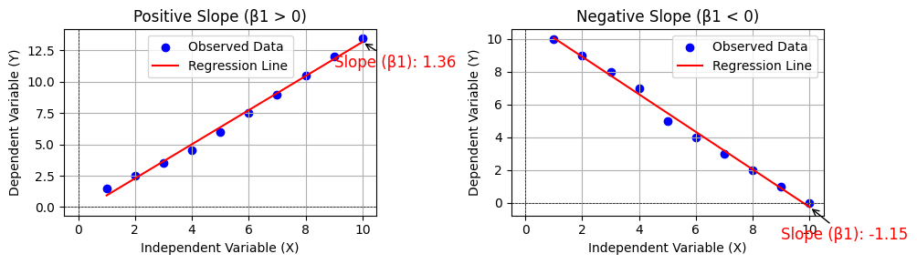
Slope \beta_1:
- A positive \beta_1 value suggests that as X increases, Y also increases, indicating a direct relationship.
- Conversely, a negative \beta_1 value indicates that an increase in X leads to a decrease in Y, indicating an inverse relationship.
For instance, if \beta_1 = 2, this would mean that for every additional unit spent on advertising, sales are expected to increase by 2 units.
Simple Linear Regression
Implementing Simple Linear Regression in Python
In order to use Simple Linear Regression in Python we must first install Python and a few necessary libraries. The fundamental setup tasks are listed below:
- **Install Python: You can download and install Python from the official Python website.
- **Install required libraries: Use pip (Python’s package installer) to install the necessary libraries, such as numpy, pandas, matplotlib, and scikit-learn.
**pip install numpy pandas matplotlib scikit-learn
This configuration will set up the environment for Python machine learning modelling, data processing, and visualization.
We will use an actual dataset to demonstrate how to use basic linear regression. We'll be using the Boston Housing Dataset. This dataset provides details on Boston real estate costs as well as room counts, crime rates and other attributes. Based on the number of rooms we will forecast the cost of the house.
Step 1: Import Required Libraries
Python `
Import necessary libraries
import numpy as np import pandas as pd import matplotlib.pyplot as plt from sklearn.model_selection import train_test_split from sklearn.linear_model import LinearRegression from sklearn.metrics import mean_squared_error, r2_score from sklearn.datasets import load_boston
`
Step 2: Load and Explore the Dataset
We will load the dataset check its structure and examine a few sample records.
Python `
Load the Boston Housing dataset
boston = load_boston() df = pd.DataFrame(boston.data, columns=boston.feature_names)
Add the target variable (house prices) to the DataFrame
df['PRICE'] = boston.target
Display the first few rows of the dataset
print(df.head())
Check for missing values
print(df.isnull().sum())
`
**Output:
CRIM ZN INDUS CHAS NOX RM AGE DIS RAD TAX \ 0 0.00632 18.0 2.31 0.0 0.538 6.575 65.2 4.0900 1.0 296.0
1 0.02731 0.0 7.07 0.0 0.469 6.421 78.9 4.9671 2.0 242.0
2 0.02729 0.0 7.07 0.0 0.469 7.185 61.1 4.9671 2.0 242.0
3 0.03237 0.0 2.18 0.0 0.458 6.998 45.8 6.0622 3.0 222.0
4 0.06905 0.0 2.18 0.0 0.458 7.147 54.2 6.0622 3.0 222.0
PTRATIO B LSTAT PRICE
0 15.3 396.90 4.98 24.0
1 17.8 396.90 9.14 21.6
2 17.8 392.83 4.03 34.7
3 18.7 394.63 2.94 33.4
4 18.7 396.90 5.33 36.2
CRIM 0
ZN 0
INDUS 0
CHAS 0
NOX 0
RM 0
AGE 0
DIS 0
RAD 0
TAX 0
PTRATIO 0
B 0
LSTAT 0
PRICE 0
dtype: int64
**In this dataset:
- **CRIM: per capita crime rate by town
- **ZN: proportion of residential land zoned for lots over 25,000 sq. ft.
- **RM: average number of rooms per dwelling
- **PRICE: median value of owner-occupied homes in $1000s (this is our target variable)
Step 3: Selecting Features and Splitting the Data
We will use the number of rooms (RM) as the independent variable and predict house prices (PRICE). Next, we'll split the data into training and testing sets.
Python `
Define the feature (independent variable) and target (dependent variable)
X = df[['RM']] # Number of rooms y = df['PRICE'] # House prices
Split the data into training and testing sets (80% train, 20% test)
X_train, X_test, y_train, y_test = train_test_split(X, y, test_size=0.2, random_state=42)
print(f"Training set size: {X_train.shape[0]}") print(f"Testing set size: {X_test.shape[0]}")
`
**Output:
Training set size: 404
Testing set size: 102
Step 4: Train the Simple Linear Regression Model
Now we can create a Linear Regression model using scikit-learn and train it on the training data. The model will calculate the intercept (𝛽0) and coefficient (𝛽1) of the linear equation.
Python `
Create a Linear Regression model
model = LinearRegression()
Train the model on the training data
model.fit(X_train, y_train)
Print the intercept and coefficient
print(f"Intercept: {model.intercept_}") print(f"Coefficient: {model.coef_}")
`
**Output:
Intercept: -36.24631889813792
Coefficient: [9.34830141]
Step 5: Make Predictions
Once the model is trained, we can use it to make predictions on the test data.
Python `
Predict house prices for the test set
y_pred = model.predict(X_test)
Display the first few predictions alongside the actual values
predictions = pd.DataFrame({'Actual': y_test, 'Predicted': y_pred}) print(predictions.head())
`
**Output:
Actual Predicted 173 23.6 23.732383
274 32.4 26.929502
491 13.6 19.684568
72 22.8 20.451129
452 16.1 22.619935
Step 6: Visualize the Regression Line
A good way to understand the relationship between the predicted and actual data is to visualize it. We'll plot the regression line along with the actual data points.
Python `
Plot the actual data points
plt.scatter(X_test, y_test, color='blue', label='Actual')
Plot the regression line
plt.plot(X_test, y_pred, color='red', label='Regression Line')
Add labels and title
plt.xlabel('Number of Rooms (RM)') plt.ylabel('House Price ($1000s)') plt.title('Simple Linear Regression: Number of Rooms vs. House Price') plt.legend() plt.show()
`
**Output:
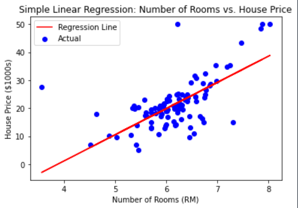
Simple Linear Regression in Python
Step 7: Evaluate the Model
Finally, we will evaluate the model's performance using metrics such as **Mean Squared Error (MSE) and **R-squared score.
Python `
Calculate Mean Squared Error (MSE)
mse = mean_squared_error(y_test, y_pred) print(f"Mean Squared Error: {mse}")
Calculate R-squared score
r2 = r2_score(y_test, y_pred) print(f"R-squared score: {r2}")
`
**Output:
Mean Squared Error: 46.144775347317264
R-squared score: 0.3707569232254778
In this tutorial we used the scikit-learn framework and Python to develop Simple Linear Regression on the Boston Housing Dataset. We used measures like Mean Squared Error (MSE) and R-squared score to assess the model's performance and forecast house prices based on the number of rooms.