Support Vector Machine (SVM) Algorithm (original) (raw)

Support Vector Machine (SVM) is a supervised machine learning algorithm used for classification and regression tasks. It tries to find the best boundary known as hyperplane that separates different classes in the data. It is useful when you want to do binary classification like spam vs. not spam or cat vs. dog.

The main goal of SVM is to maximize the margin between the two classes. The larger the margin the better the model performs on new and unseen data.

**Key Concepts of Support Vector Machine

• **Hyperplane: A decision boundary separating different classes in feature space and is represented by the equation wx + b = 0 in linear classification.
• **Support Vectors: The closest data points to the hyperplane, crucial for determining the hyperplane and margin in SVM.
• **Margin: The distance between the hyperplane and the support vectors. SVM aims to maximize this margin for better classification performance.
• **Kernel: A function that maps data to a higher-dimensional space enabling SVM to handle non-linearly separable data.
• **Hard Margin: A maximum-margin hyperplane that perfectly separates the data without misclassifications.
• **Soft Margin: Allows some misclassifications by introducing slack variables, balancing margin maximization and misclassification penalties when data is not perfectly separable.
• **C: A regularization term balancing margin maximization and misclassification penalties. A higher C value forces stricter penalty for misclassifications.
• **Hinge Loss: A loss function penalizing misclassified points or margin violations and is combined with regularization in SVM.
• **Dual Problem: Involves solving for Lagrange multipliers associated with support vectors, facilitating the kernel trick and efficient computation.

How does Support Vector Machine Algorithm Work?

The key idea behind the SVM algorithm is to find the hyperplane that best separates two classes by maximizing the margin between them. This margin is the distance from the hyperplane to the nearest data points (support vectors) on each side.

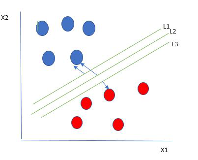
Multiple hyperplanes separate the data from two classes

The best hyperplane also known as the ****"hard margin"** is the one that maximizes the distance between the hyperplane and the nearest data points from both classes. This ensures a clear separation between the classes. So from the above figure, we choose L2 as hard margin. Let's consider a scenario like shown below:

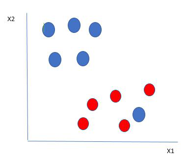
Selecting hyperplane for data with outlier

Here, we have one blue ball in the boundary of the red ball.

**How does SVM classify the data?

The blue ball in the boundary of red ones is an outlier of blue balls. The SVM algorithm has the characteristics to ignore the outlier and finds the best hyperplane that maximizes the margin. SVM is robust to outliers.

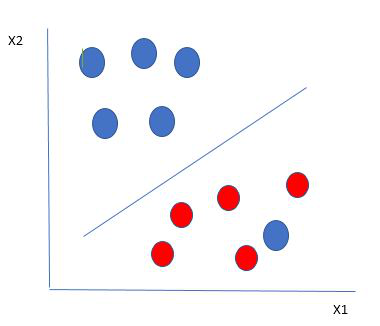
Hyperplane which is the most optimized one

A soft margin allows for some misclassifications or violations of the margin to improve generalization. The SVM optimizes the following equation to balance margin maximization and penalty minimization:

\text{Objective Function} = (\frac{1}{\text{margin}}) + \lambda \sum \text{penalty }

The penalty used for violations is often hinge loss which has the following behavior:

• If a data point is correctly classified and within the margin there is no penalty (loss = 0).
• If a point is incorrectly classified or violates the margin the hinge loss increases proportionally to the distance of the violation.

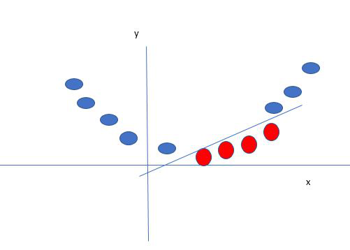
Till now we were talking about linearly separable data that seprates group of blue balls and red balls by a straight line/linear line.

**What to do if data are not linearly separable?

When data is not linearly separable i.e it can't be divided by a straight line, SVM uses a technique called kernels to map the data into a higher-dimensional space where it becomes separable. This transformation helps SVM find a decision boundary even for non-linear data.

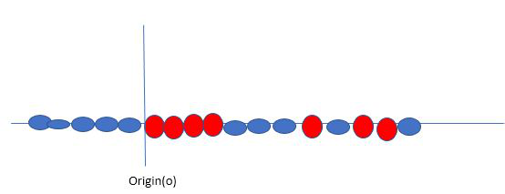
Original 1D dataset for classification

A kernel is a function that maps data points into a higher-dimensional space without explicitly computing the coordinates in that space. This allows SVM to work efficiently with non-linear data by implicitly performing the mapping. For example consider data points that are not linearly separable. By applying a kernel function SVM transforms the data points into a higher-dimensional space where they become linearly separable.

• **Linear Kernel: For linear separability.
• **Polynomial Kernel: Maps data into a polynomial space.
• **Radial Basis Function (RBF) Kernel: Transforms data into a space based on distances between data points.

Mapping 1D data to 2D to become able to separate the two classes

In this case the new variable y is created as a function of distance from the origin.

Mathematical Computation of SVM

Consider a binary classification problem with two classes, labeled as +1 and -1. We have a training dataset consisting of input feature vectors X and their corresponding class labels Y. The equation for the linear hyperplane can be written as:

w^Tx+ b = 0

Where:

• w is the normal vector to the hyperplane (the direction perpendicular to it).
• b is the offset or bias term representing the distance of the hyperplane from the origin along the normal vector w.

Distance from a Data Point to the Hyperplane

The distance between a data point x_i and the decision boundary can be calculated as:

d_i = \frac{w^T x_i + b}{||w||}

where ||w|| represents the Euclidean norm of the weight vector w. Euclidean norm of the normal vector W

Linear SVM Classifier

Distance from a Data Point to the Hyperplane:

\hat{y} = \left\{ \begin{array}{cl} 1 & : \ w^Tx+b \geq 0 \\ 0 & : \ w^Tx+b < 0 \end{array} \right.

Where \hat{y} is the predicted label of a data point.

**Optimization Problem for SVM

For a linearly separable dataset the goal is to find the hyperplane that maximizes the margin between the two classes while ensuring that all data points are correctly classified. This leads to the following optimization problem:

\underset{w,b}{\text{minimize}}\frac{1}{2}\left\| w \right\|^{2}

Subject to the constraint:

y_i(w^Tx_i + b) \geq 1 \;for\; i = 1, 2,3, \cdots,m

Where:

• y_i​ is the class label (+1 or -1) for each training instance.
• x_i​ is the feature vector for the i-th training instance.
• m is the total number of training instances.

The condition y_i (w^T x_i + b) \geq 1 ensures that each data point is correctly classified and lies outside the margin.

**Soft Margin in Linear SVM Classifier

In the presence of outliers or non-separable data the SVM allows some misclassification by introducing slack variables \zeta_i​. The optimization problem is modified as:

\underset{w, b}{\text{minimize }} \frac{1}{2} \|w\|^2 + C \sum_{i=1}^{m} \zeta_i

Subject to the constraints:

y_i (w^T x_i + b) \geq 1 - \zeta_i \quad \text{and} \quad \zeta_i \geq 0 \quad \text{for } i = 1, 2, \dots, m

Where:

• C is a regularization parameter that controls the trade-off between margin maximization and penalty for misclassifications.
• \zeta_i​ are slack variables that represent the degree of violation of the margin by each data point.

**Dual Problem for SVM

The dual problem involves maximizing the Lagrange multipliers associated with the support vectors. This transformation allows solving the SVM optimization using kernel functions for non-linear classification.

The dual objective function is given by:

\underset{\alpha}{\text{maximize }} \frac{1}{2} \sum_{i=1}^{m} \sum_{j=1}^{m} \alpha_i \alpha_j t_i t_j K(x_i, x_j) - \sum_{i=1}^{m} \alpha_i

Where:

• \alpha_i​ are the Lagrange multipliers associated with the i^{th} training sample.
• t_i​ is the class label for the i^{th} -th training sample.
• K(x_i, x_j) is the kernel function that computes the similarity between data points x_i​ and x_j​. The kernel allows SVM to handle non-linear classification problems by mapping data into a higher-dimensional space.

The dual formulation optimizes the Lagrange multipliers \alpha_i​ and the support vectors are those training samples where \alpha_i > 0.

**SVM Decision Boundary

Once the dual problem is solved, the decision boundary is given by:

w = \sum_{i=1}^{m} \alpha_i t_i K(x_i, x) + b

Where w is the weight vector, x is the test data point and b is the bias term. Finally the bias term b is determined by the support vectors, which satisfy:

t_i (w^T x_i - b) = 1 \quad \Rightarrow \quad b = w^T x_i - t_i

Where x_i​ is any support vector.

This completes the mathematical framework of the Support Vector Machine algorithm which allows for both linear and non-linear classification using the dual problem and kernel trick.

Types of Support Vector Machine

Based on the nature of the decision boundary, Support Vector Machines (SVM) can be divided into two main parts:

• **Linear SVM: Linear SVMs use a linear decision boundary to separate the data points of different classes. When the data can be precisely linearly separated, linear SVMs are very suitable. This means that a single straight line (in 2D) or a hyperplane (in higher dimensions) can entirely divide the data points into their respective classes. A hyperplane that maximizes the margin between the classes is the decision boundary.
• **Non-Linear SVM: Non-Linear SVM can be used to classify data when it cannot be separated into two classes by a straight line (in the case of 2D). By using kernel functions, nonlinear SVMs can handle nonlinearly separable data. The original input data is transformed by these kernel functions into a higher-dimensional feature space where the data points can be linearly separated. A linear SVM is used to locate a nonlinear decision boundary in this modified space.

**Implementing SVM Algorithm in Python

Predict if cancer is Benign or malignant. Using historical data about patients diagnosed with cancer enables doctors to differentiate malignant cases and benign ones are given independent attributes.

• Load the breast cancer dataset from sklearn.datasets
• Separate input features and target variables.
• Build and train the SVM classifiers using RBF kernel.
• Plot the scatter plot of the input features. Python `

Load the important packages

from sklearn.datasets import load_breast_cancer import matplotlib.pyplot as plt from sklearn.inspection import DecisionBoundaryDisplay from sklearn.svm import SVC

Load the datasets

cancer = load_breast_cancer() X = cancer.data[:, :2] y = cancer.target

#Build the model svm = SVC(kernel="rbf", gamma=0.5, C=1.0)

Trained the model

svm.fit(X, y)

Plot Decision Boundary

DecisionBoundaryDisplay.from_estimator( svm, X, response_method="predict", cmap=plt.cm.Spectral, alpha=0.8, xlabel=cancer.feature_names[0], ylabel=cancer.feature_names[1], )

Scatter plot

plt.scatter(X[:, 0], X[:, 1], c=y, s=20, edgecolors="k") plt.show()

`

**Output:

Breast Cancer Classifications with SVM RBF kernel

**Advantages of Support Vector Machine (SVM)

1. **High-Dimensional Performance: SVM excels in high-dimensional spaces, making it suitable for image classification and gene expression analysis.
2. **Nonlinear Capability: Utilizing kernel functions like RBF and polynomial SVM effectively handles nonlinear relationships.
3. **Outlier Resilience: The soft margin feature allows SVM to ignore outliers, enhancing robustness in spam detection and anomaly detection.
4. **Binary and Multiclass Support: SVM is effective for both binary classification and multiclass classification suitable for applications in text classification.
5. **Memory Efficiency: It focuses on support vectors making it memory efficient compared to other algorithms.

**Disadvantages of Support Vector Machine (SVM)

1. **Slow Training: SVM can be slow for large datasets, affecting performance in SVM in data mining tasks.
2. **Parameter Tuning Difficulty: Selecting the right kernel and adjusting parameters like C requires careful tuning, impacting SVM algorithms.
3. **Noise Sensitivity: SVM struggles with noisy datasets and overlapping classes, limiting effectiveness in real-world scenarios.
4. **Limited Interpretability: The complexity of the hyperplane in higher dimensions makes SVM less interpretable than other models.
5. **Feature Scaling Sensitivity: Proper feature scaling is essential, otherwise SVM models may perform poorly.