Hypothesis (language regularity) and algorithm (Lgraph to NFA) in TOC (original) (raw)

Last Updated : 10 Mar, 2026

L-graphs can generate context-sensitive languages, but programming such languages is more difficult than programming regular languages. Therefore, a hypothesis is proposed to identify the type of L-graphs that generate regular languages.A nest is a neutral path T₁ T₂ T₃ where T₁ and T₃ are cycles and T₂ is a neutral path connecting them. This path is called an iterating nest if all three paths print repetitions of the same string α.

Points defining an iterating nest:

1. T₁ prints αᵏ
2. T₂ prints αˡ
3. T₃ prints αᵐ
4. k, l, m ≥ 0
5. α is a string of input symbols
6. At least one of k, l, or m should be ≥ 1

Hypothesis: If all nests in a context-free L-graph G are iterating nests, then the language L(G) generated by G is a regular language. Based on this hypothesis, such L-graphs can be converted into an equivalent NFA.

• **Step-1: Languages of the L-graph and NFA must be the same, thusly, we won’t need a new alphabet \Rightarrow \Sigma’’ = \Sigma, \: P’’ = P . (Comment: we build context free L-graph G’’, which is equal to the start graph G’, with no conflicting nests)
• **Step-2: Build Core(1, 1) for the graph G. V’’ := {(v, \varepsilon ) | v \in V of \forall canon k \in Core(1, 1), v \notin k} \lambda'' := { arcs o \in \lambda | start and final states o', o'' \in V’’} For all k \in Core(1, 1): Step 1’. v := 1st state of canon k. \eta := \varepsilon . V’’ \cup= (v, \eta) Step 2’. \lambda'' \cup= arc from state (v, \eta) followed this arc into new state defined with following rules: \eta := \eta , if the input bracket on this arc = \varepsilon ; \eta'the\: input\: bracket' , if the input bracket is an opening one; \eta 'without\: the\: last\: bracket' , if the input bracket is a closing bracket v := 2nd state of canon k V’’ \cup= (v, \eta) Step 3’. Repeat Step 2’, while there are still arcs in the canon.
• **Step-3: Build Core(1, 2). If the canon has 2 equal arcs in a row: the start state and the final state match; we add the arc from given state into itself, using this arc, to \lambda'' . Add the remaining in \lambda arcs v – u (\alpha) to \lambda'' in the form of (v, \varepsilon) - (u, \varepsilon) (\alpha)
• **Step-4: P''_0 = (P_0, \varepsilon).\: F'' = \{(f, \varepsilon) | f \in F\} (Comment: following is an algorithm of converting context free L-graph G’’ into NFA G’)
• **Step-5: Do the following to every iterating complement T = T_1T_2T_3 in G’’: Add a new state v. Create a path that starts in state beg(T_3) , equal to T_3 . From v into T_3 create the path, equal to T_1 . Delete cycles T_1 and T_3 .
• **Step-6: G’ = G’’, where arcs are not loaded with brackets.

So that every step above is clear I’m showing you the next example. \textbf{Example:}\\ \textbf{Input:} Context free L-graph with iterating complements G = ( \{a, b, c\}, \\*\{1, 2, 3\} \\*\{( (, ) ), ( [, ] )\}, \\*\\*\{ (: \{ 1 – a – 1 \}, \\*): \{ 2 – a – 2 \}, \\*\big[: \{ 1 – b – 2 \}, \\*\big]: \{ 2 – c – 3 \}, \\*\varepsilon: \{ 1 – a – 2 \} \}, \\*\\*1, \\*\{2, 3\} \} , which determines the language = \{a^(^2^n^+^1^) | n \geqslant 0\} \cup \{bc\} Start graph G \Sigma'' = \{a, b, c\}\\ V’’ = \varnothing\\ \lambda’’ = \varnothing Core(1, 1) = { 1 – a – 2 ; 1 – a, (1 – 1 – a – 2 – a, )1 – 2 ; 1 – b, (2 – 2 – c, )2 – 3 } Core(1, 2) = Core(1, 1) \cup { 1 – a, (1 – 1 – a, (1 – 1 – a – 2 – a, )1 – 2 – a, )1 – 2 } Step 2: Step 1’ – Step 3’ \Rightarrow\\ V’’ = \{(1, \varepsilon), (2, (_2), (3, \varepsilon), (1, (_1), (2, )_1), (2, \varepsilon)\}\\* \lambda’’ = \{ \\*(: \{ (1, \varepsilon) – a – (1, (); (1, () – a – (1, () \}, \\*): \{ (2, )) – a – (2, )); (2, )) – a – (2, \varepsilon) \}, \\*\big[: \{ (1, \varepsilon) – b – (2, [) \}, \\*\big]: \{ (2, [) – c – (3, \varepsilon) \}, \\*\varepsilon: \{ (1, \varepsilon) – a – (2, \varepsilon); (1, () – a – (2, )) \} \}\\ P’’_0 = (1, \varepsilon)\\ F’’ = \{(2, \varepsilon), (3, \varepsilon)\}\\ G’’ = (\Sigma’’, V’’, P’’, \lambda’’, P’’_0, F’’) 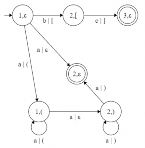Intermediate graph G’’ \Sigma’ = \{a, b, c\}\\ V’ = V’’ \cup \{4\}\\ P’_0 = P’’_0\\ F’ = F’’\\ \lambda’ = \{ \\*(1, \varepsilon) – a – (1, (); \\*(2, )) – a – 4; \\*4 – a – (2, )); \\*(2, )) – a – (2, \varepsilon); \\*(1, \varepsilon) – b – (2, [); \\*(2, [) – c – (3, \varepsilon); \\*(1, \varepsilon) – a – (2, \varepsilon); \\*(1, () – a – (2, )) \}\\ G’ = (\Sigma’, V’, \lambda’, P’_0, F’) 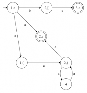NFA G’

Advantages of hypotheses

• **Framework for analysis: Hypotheses about language regularity provide a structured way to analyze and classify languages into classes such as regular and context-free.
• **Understanding language behavior: They help researchers understand how languages behave. For example, regular languages have clear properties and can be recognized using finite automata.
• **Bridging theory and practice: These hypotheses connect theoretical concepts with practical applications like compiler design, pattern matching, and text processing.

Disadvantages of hypotheses

• **Limitations of classification: Not all languages fit clearly into predefined classes like regular or context-free, which makes classification difficult.
• **Complex languages: Many real-world applications involve complex languages such as context-free or context-sensitive languages where the regularity assumption may not work.
• **Oversimplification: Assuming a language is regular can oversimplify the problem and may ignore important structural properties of the language.