Vanishing and Exploding Gradients Problems in Deep Learning (original) (raw)

In the realm of deep learning, the optimization process plays a crucial role in training neural networks. Gradient descent, a fundamental optimization algorithm, can sometimes encounter two common issues: vanishing gradients and exploding gradients. In this article, we will delve into these challenges, providing insights into what they are, why they occur, and how to mitigate them. We will build and train a model, and learn how to face vanishing and exploding problems.

What is Vanishing Gradient?

The vanishing gradient problem is a challenge that emerges during backpropagation when the derivatives or slopes of the activation functions become progressively smaller as we move backward through the layers of a neural network. This phenomenon is particularly prominent in deep networks with many layers, hindering the effective training of the model. The weight updates becomes extremely tiny, or even exponentially small, it can significantly prolong the training time, and in the worst-case scenario, it can halt the training process altogether.

Why the Problem Occurs?

During backpropagation, the gradients propagate back through the layers of the network, they decrease significantly. This means that as they leave the output layer and return to the input layer, the gradients become progressively smaller. As a result, the weights associated with the initial levels, which accommodate these small gradients, are updated little or not at each iteration of the optimization process.

**The vanishing gradient problem is particularly associated with the sigmoid and hyperbolic tangent (tanh) activation functions because their derivatives fall within the range of 0 to 0.25 and 0 to 1, respectively. Consequently, extreme weights becomes very small, causing the updated weights to closely resemble the original ones. This persistence of small updates contributes to the vanishing gradient issue.

The sigmoid and tanh functions limit the input values ​​to the ranges [0,1] and [-1,1], so that they saturate at 0 or 1 for sigmoid and -1 or 1 for Tanh. The derivatives at points becomes zero as they are moving. In these regions, especially when inputs are very small or large, the gradients are very close to zero. While this may not be a major concern in shallow networks with a few layers, it is a more pronounced issue in deep networks. When the inputs fall in saturated regions, the gradients approach zero, resulting in little update to the weights of the previous layer. In simple networks this does not pose much of a problem, but as more layers are added, these small gradients, which multiply between layers, decay significantly and consequently the first layer tears very slowly , and hinders overall model performance and can lead to convergence failure.

How can we identify?

Identifying the vanishing gradient problem typically involves monitoring the training dynamics of a deep neural network.

• One key indicator is observing model weights converging to 0 or stagnation in the improvement of the model's performance metrics over training epochs.
• During training, if the **loss function fails to decrease significantly, or if there is erratic behavior in the learning curves, it suggests that the gradients may be vanishing.
• Additionally, examining the gradients themselves during backpropagation can provide insights. **Visualization techniques, such as gradient histograms or norms, can aid in assessing the distribution of gradients throughout the network.

How can we solve the issue?

• **Batch Normalization : Batch normalization normalizes the inputs of each layer, reducing internal covariate shift. This can help stabilize and accelerate the training process, allowing for more consistent gradient flow.
• **Activation function: Activation function like **Rectified Linear Unit (ReLU) can be used. With **ReLU, the gradient is 0 for negative and zero input, and it is 1 for positive input, which helps alleviate the vanishing gradient issue. Therefore, ReLU operates by replacing poor enter values with 0, and 1 for fine enter values, it preserves the input unchanged.
• **Skip Connections and Residual Networks (ResNets): Skip connections, as seen in ResNets, allow the gradient to bypass certain layers during backpropagation. This facilitates the flow of information through the network, preventing gradients from vanishing.
• **Long Short-Term Memory Networks (LSTMs) and Gated Recurrent Units (GRUs): In the context of recurrent neural networks (RNNs), architectures like LSTMs and GRUs are designed to address the vanishing gradient problem in sequences by incorporating gating mechanisms .
• **Gradient Clipping: Gradient clipping involves imposing a threshold on the gradients during backpropagation. Limit the magnitude of gradients during backpropagation, this can prevent them from becoming too small or exploding, which can also hinder learning.

Build and train a model for Vanishing Gradient Problem

let's see how the problems occur , and way to handle them.

**Step 1: Import Libraries

First, import the necessary libraries for model

Python `

import matplotlib.pyplot as plt import numpy as np import pandas as pd import tensorflow as tf import keras from sklearn.model_selection import train_test_split from keras.layers import Dense from keras.models import Sequential import seaborn as sns from imblearn.over_sampling import RandomOverSampler from keras.layers import Dense, Dropout from keras.optimizers import Adam from keras.callbacks import EarlyStopping from sklearn.preprocessing import StandardScaler from sklearn.metrics import classification_report from keras.initializers import random_normal from keras.constraints import max_norm from keras.optimizers import SGD

`

Step 2: Loading dataset

The code loads two CSV files (Credit_card.csv and Credit_card_label.csv) into Pandas DataFrames, df and labels.

Link to dataset: Credit card details Binary classification.

Python `

df = pd.read_csv('/content/Credit_card.csv') labels = pd.read_csv('/content/Credit_card_label.csv')

`

Step 3: Data Preprocessing

We create a new column 'Approved' in the DataFrame by converting the 'label' column from the 'labels' DataFrame to integers.

Python `

dep = 'Approved'

df[dep] = labels.label.astype(int)

df.loc[df[dep] == 1, 'Status'] = 'Approved' df.loc[df[dep] == 0, 'Status'] = 'Declined'

`

Step 4: Feature Engineering

We perform some feature engineering on the data, creating new columns 'Age', 'EmployedDaysOnly', and 'UnemployedDaysOnly' based on existing columns.

It converts categorical variables in the 'cats' list to numerical codes using pd.Categorical and fills missing values with the mode of each column.

Python `

cats = [ 'GENDER', 'Car_Owner', 'Propert_Owner', 'Type_Income', 'EDUCATION', 'Marital_status', 'Housing_type', 'Mobile_phone', 'Work_Phone', 'Phone', 'Type_Occupation', 'EMAIL_ID' ]

conts = [ 'CHILDREN', 'Family_Members', 'Annual_income', 'Age', 'EmployedDaysOnly', 'UnemployedDaysOnly' ] def proc_data(): df['Age'] = -df.Birthday_count // 365 df['EmployedDaysOnly'] = df.Employed_days.apply(lambda x: x if x > 0 else 0) df['UnemployedDaysOnly'] = df.Employed_days.apply(lambda x: abs(x) if x < 0 else 0)

for cat in cats:
    df[cat] = pd.Categorical(df[cat])

modes = df.mode().iloc[0]
df.fillna(modes, inplace=True)

proc_data()

`

Step 5: Oversampling due to heavily skewed data and Data Splitting

Python `

X = df[cats + conts] y = df[dep]
X_over, y_over = RandomOverSampler().fit_resample(X, y)

X_train, X_val, y_train, y_val = train_test_split(X_over, y_over, test_size=0.25)

`

Step 6: Encoding

The code applies the cat.codes method to each column specified in the cats list. The method is applicable to Pandas categorical data types and assigns a unique numerical code to each unique category in the categorical variable. The result is that the categorical variables are replaced with their corresponding numerical codes.

Python `

X_train[cats] = X_train[cats].apply(lambda x: x.cat.codes) X_val[cats] = X_val[cats].apply(lambda x: x.cat.codes)

`

Step 7: Model Creation

Create a Sequential model using Keras. A Sequential model allows you to build a neural network by stacking layers one after another.

Python `

model = Sequential()

`

Step 8: Adding layers

Adding 10 dense layers to the model. Each dense layer has 10 units (neurons) and uses the sigmoid activation function. The first layer specifies input_dim=18, indicating that the input data has 18 features. This is the input layer. The last layer has a single neuron and uses sigmoid activation, making it suitable for binary classification tasks.

Python `

model.add(Dense(10, activation='sigmoid', input_dim=18)) model.add(Dense(10, activation='sigmoid')) model.add(Dense(10, activation='sigmoid')) model.add(Dense(10, activation='sigmoid')) model.add(Dense(10, activation='sigmoid')) model.add(Dense(10, activation='sigmoid')) model.add(Dense(10, activation='sigmoid')) model.add(Dense(10, activation='sigmoid')) model.add(Dense(10, activation='sigmoid')) model.add(Dense(1, activation='sigmoid'))

`

Step 9: Model Compilation

This step specifies the loss function, optimizer, and evaluation metrics.

Python `

model.compile(loss='binary_crossentropy', optimizer='adam', metrics=['accuracy'])

`

Step 10: Model training

Train the model using the training data (X_train and y_train) for 100 epochs.The training history is stored in the history object, which contains information about the training process, including loss and accuracy at each epoch.

Python `

history = model.fit(X_train, y_train, epochs=100)

`

**Output:

Epoch 1/100
65/65 [==============================] - 3s 3ms/step - loss: 0.7027 - accuracy: 0.5119
Epoch 2/100
65/65 [==============================] - 0s 3ms/step - loss: 0.6936 - accuracy: 0.5119
Epoch 3/100
65/65 [==============================] - 0s 3ms/step - loss: 0.6933 - accuracy: 0.5119
.
.
Epoch 97/100
65/65 [==============================] - 0s 3ms/step - loss: 0.6930 - accuracy: 0.5119
Epoch 98/100
65/65 [==============================] - 0s 3ms/step - loss: 0.6930 - accuracy: 0.5119
Epoch 99/100
65/65 [==============================] - 0s 3ms/step - loss: 0.6932 - accuracy: 0.5119
Epoch 100/100
65/65 [==============================] - 0s 3ms/step - loss: 0.6929 - accuracy: 0.5119

Step 11: Plotting the training loss

Python `

loss = history.history['loss'] epochs = range(1, len(loss) + 1) plt.plot(epochs, loss, 'b', label='Training Loss') plt.title('Training Loss') plt.xlabel('Epochs') plt.ylabel('Loss') plt.legend() plt.show()

`

**Output:

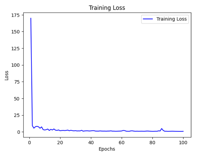
Loss does not change much as gradient becomes too small

Solution for Vanishing Gradient Problem

Step 1: Scaling

Python `

scaler = StandardScaler() X_train_scaled = scaler.fit_transform(X_train) X_val_scaled = scaler.transform(X_val)

`

Step 2: Modify the Model

1. Deeper Architecture: Augment model with more layers with increased numbers of neurons in each layer. Deeper architectures can capture more complex relationships in the data.
2. Early Stopping: Early stopping is implemented to monitor the validation loss. Training will stop if the validation loss does not improve for a certain number of epochs (defined by patience).
3. Increased Dropout: Dropout layers are added after each dense layer to help prevent overfitting.
4. Adjusting Learning Rate: The learning rate is set to 0.001. You can experiment with different learning rates. Python `

model2 = Sequential()

model2.add(Dense(128, activation='relu', input_dim=18)) model2.add(Dropout(0.5)) model2.add(Dense(256, activation='relu')) model2.add(Dropout(0.5)) model2.add(Dense(128, activation='relu')) model2.add(Dropout(0.5)) model2.add(Dense(64, activation='relu')) model2.add(Dropout(0.5)) model2.add(Dense(1, activation='sigmoid'))

early_stopping = EarlyStopping(monitor='val_loss', patience=10, restore_best_weights=True)

model2.compile(loss='binary_crossentropy', optimizer=Adam(learning_rate=0.001), metrics=['accuracy'])

history2 = model2.fit(X_train_scaled, y_train, epochs=100, validation_data=(X_val_scaled, y_val), batch_size=32, callbacks=[early_stopping])

`

**Output:

Epoch 1/100
65/65 [==============================] - 3s 8ms/step - loss: 0.7167 - accuracy: 0.5308 - val_loss: 0.6851 - val_accuracy: 0.5590
Epoch 2/100
65/65 [==============================] - 0s 5ms/step - loss: 0.6967 - accuracy: 0.5367 - val_loss: 0.6771 - val_accuracy: 0.6259
Epoch 3/100
65/65 [==============================] - 0s 5ms/step - loss: 0.6879 - accuracy: 0.5488 - val_loss: 0.6767 - val_accuracy: 0.5721
Epoch 4/100
65/65 [==============================] - 0s 5ms/step - loss: 0.6840 - accuracy: 0.5673 - val_loss: 0.6628 - val_accuracy: 0.6114
.
.
Epoch 96/100
65/65 [==============================] - 0s 7ms/step - loss: 0.1763 - accuracy: 0.9349 - val_loss: 0.1909 - val_accuracy: 0.9301
Epoch 97/100
65/65 [==============================] - 0s 7ms/step - loss: 0.1653 - accuracy: 0.9325 - val_loss: 0.1909 - val_accuracy: 0.9345
Epoch 98/100
65/65 [==============================] - 1s 8ms/step - loss: 0.1929 - accuracy: 0.9237 - val_loss: 0.1975 - val_accuracy: 0.9229
Epoch 99/100
65/65 [==============================] - 1s 9ms/step - loss: 0.1846 - accuracy: 0.9281 - val_loss: 0.1904 - val_accuracy: 0.9330
Epoch 100/100
65/65 [==============================] - 0s 7ms/step - loss: 0.1885 - accuracy: 0.9228 - val_loss: 0.1981 - val_accuracy: 0.9330

Evaluation metrics

Python `

predictions = model2.predict(X_val_scaled) rounded_predictions = np.round(predictions) report = classification_report(y_val, rounded_predictions) print(f'Classification Report:\n{report}')

`

**Output:

22/22 [==============================] - 0s 2ms/step
Classification Report:
precision recall f1-score support
0 1.00 0.87 0.93 352
1 0.88 1.00 0.94 335
accuracy **0.93 687
macro avg 0.94 0.93 0.93 687
weighted avg 0.94 0.93 0.93 687

What is Exploding Gradient?

The exploding gradient problem is a challenge encountered during training deep neural networks. It occurs when the gradients of the network's loss function with respect to the weights (parameters) become excessively large.

Why Exploding Gradient Occurs?

The issue of exploding gradients arises when, during backpropagation, the derivatives or slopes of the neural network's layers grow progressively larger as we move backward. This is essentially the opposite of the vanishing gradient problem.

The root cause of this problem lies in the weights of the network, rather than the choice of activation function. High weight values lead to correspondingly high derivatives, causing significant deviations in new weight values from the previous ones. As a result, the gradient fails to converge and can lead to the network oscillating around local minima, making it challenging to reach the global minimum point.

In summary, exploding gradients occur when weight values lead to excessively large derivatives, making convergence difficult and potentially preventing the neural network from effectively learning and optimizing its parameters.

As we discussed earlier, the update for the weights during backpropagation in a neural network is given by:

\Delta W_i = -\alpha \cdot \frac{\partial L}{\partial W_i}

where,

• ΔW_i : The change in the weight W_i
• **α: The learning rate, a hyperparameter that controls the step size of the update.
• **L: The loss function that measures the error of the model.
• \frac{∂L}{∂W_i}: The partial derivative of the loss function with respect to the weight W_i, which indicates the gradient of the loss function with respect to that weight.

The exploding gradient problem occurs when the gradients become very large during backpropagation. This is often the result of gradients greater than 1, leading to a rapid increase in values as you propagate them backward through the layers.

Mathematically, the update rule becomes problematic when∣∇W_i∣>1, causing the weights to increase exponentially during training.

How can we identify the problem?

Identifying the presence of exploding gradients in deep neural network requires careful observation and analysis during training. Here are some key indicators:

• The loss function exhibits erratic behavior, oscillating wildly instead of steadily decreasing suggesting that the network weights are being updated excessively by large gradients, preventing smooth convergence.
• The training process encounters "NaN" (Not a Number) values in the loss function or other intermediate calculations..
• If network weights, during training exhibit significant and rapid increases in their values, it suggests the presence of exploding gradients.
• Tools like TensorBoard can be used to visualize the gradients flowing through the network.

How can we solve the issue?

• **Gradient Clipping: It sets a maximum threshold for the magnitude of gradients during backpropagation. Any gradient exceeding the threshold is clipped to the threshold value, preventing it from growing unbounded.
• **Batch Normalization: This technique normalizes the activations within each mini-batch, effectively scaling the gradients and reducing their variance. This helps prevent both vanishing and exploding gradients, improving stability and efficiency.

Build and train a model for Exploding Gradient Problem

We work on the same preprocessed data from the Vanishing gradient example but define a different neural network.

Step 1: Model creation and adding layers

Python `

model = Sequential()

model.add(Dense(10, activation='tanh', kernel_initializer=random_normal(mean=0.0, stddev=1.0), input_dim=18)) model.add(Dense(10, activation='tanh', kernel_initializer=random_normal(mean=0.0, stddev=1.0))) model.add(Dense(10, activation='tanh', kernel_initializer=random_normal(mean=0.0, stddev=1.0))) model.add(Dense(10, activation='tanh', kernel_initializer=random_normal(mean=0.0, stddev=1.0))) model.add(Dense(10, activation='tanh', kernel_initializer=random_normal(mean=0.0, stddev=1.0))) model.add(Dense(10, activation='tanh', kernel_initializer=random_normal(mean=0.0, stddev=1.0))) model.add(Dense(10, activation='tanh', kernel_initializer=random_normal(mean=0.0, stddev=1.0))) model.add(Dense(10, activation='tanh', kernel_initializer=random_normal(mean=0.0, stddev=1.0))) model.add(Dense(1, activation='sigmoid'))

`

Step 2: Model compiling

Python `

optimizer = SGD(learning_rate=1.0) model.compile(loss='binary_crossentropy', optimizer=optimizer, metrics=['accuracy'])

`

Step 3: Model training

Python `

history = model.fit(X_train, y_train, epochs=100)

`

**Output:

Epoch 1/100
65/65 [==============================] - 2s 5ms/step - loss: 0.7919 - accuracy: 0.5032
Epoch 2/100
65/65 [==============================] - 0s 4ms/step - loss: 0.7440 - accuracy: 0.5017
.
.
Epoch 99/100
65/65 [==============================] - 0s 4ms/step - loss: 0.7022 - accuracy: 0.5085
Epoch 100/100
65/65 [==============================] - 0s 5ms/step - loss: 0.7037 - accuracy: 0.5061

Step 4: Plotting training loss

Python `

loss = history.history['loss']
epochs = range(1, len(loss) + 1)

plt.plot(epochs, loss, 'b', label='Training Loss') plt.title('Training Loss') plt.xlabel('Epochs') plt.ylabel('Loss') plt.legend() plt.show()

`

**Output:

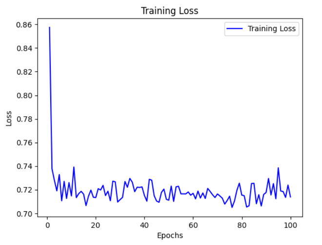
It is observed that the loss does not converge and keeps fluctuating which shows we have encountered an exploding gradient problem.

Solution for Exploding Gradient Problem

Below methods can be used to modify the model:

1. Weight Initialization: The weight initialization is changed to 'glorot_uniform,' which is a commonly used initialization for neural networks.
2. Gradient Clipping: The clipnorm parameter in the Adam optimizer is set to 1.0, which performs gradient clipping. This helps prevent exploding gradients.
3. Kernel Constraint: The max_norm constraint is applied to the kernel weights of each layer with a maximum norm of 2.0. This further helps in preventing exploding gradients. Python `

model = Sequential()

model.add(Dense(10, activation='tanh', kernel_initializer='glorot_uniform', kernel_constraint=max_norm(2.0), input_dim=18)) model.add(Dense(10, activation='tanh', kernel_initializer='glorot_uniform', kernel_constraint=max_norm(2.0))) model.add(Dense(10, activation='tanh', kernel_initializer='glorot_uniform', kernel_constraint=max_norm(2.0))) model.add(Dense(10, activation='tanh', kernel_initializer='glorot_uniform', kernel_constraint=max_norm(2.0))) model.add(Dense(10, activation='tanh', kernel_initializer='glorot_uniform', kernel_constraint=max_norm(2.0))) model.add(Dense(10, activation='tanh', kernel_initializer='glorot_uniform', kernel_constraint=max_norm(2.0))) model.add(Dense(10, activation='tanh', kernel_initializer='glorot_uniform', kernel_constraint=max_norm(2.0))) model.add(Dense(10, activation='tanh', kernel_initializer='glorot_uniform', kernel_constraint=max_norm(2.0))) model.add(Dense(1, activation='sigmoid'))

early_stopping = EarlyStopping(monitor='val_loss', patience=10, restore_best_weights=True)

model.compile(loss='binary_crossentropy', optimizer=Adam(learning_rate=0.001, clipnorm=1.0), metrics=['accuracy'])

history = model.fit(X_train_scaled, y_train, epochs=100, validation_data=(X_val_scaled, y_val), batch_size=32, callbacks=[early_stopping])

`

**Output:

Epoch 1/100
65/65 [==============================] - 6s 11ms/step - loss: 0.6865 - accuracy: 0.5537 - val_loss: 0.6818 - val_accuracy: 0.5764
Epoch 2/100
65/65 [==============================] - 1s 8ms/step - loss: 0.6608 - accuracy: 0.6202 - val_loss: 0.6746 - val_accuracy: 0.6070
Epoch 3/100
65/65 [==============================] - 1s 8ms/step - loss: 0.6440 - accuracy: 0.6357 - val_loss: 0.6624 - val_accuracy: 0.6099
.
.
Epoch 68/100
65/65 [==============================] - 1s 11ms/step - loss: 0.1909 - accuracy: 0.9257 - val_loss: 0.3819 - val_accuracy: 0.8486
Epoch 69/100
65/65 [==============================] - 1s 11ms/step - loss: 0.1811 - accuracy: 0.9286 - val_loss: 0.3533 - val_accuracy: 0.8574
Epoch 70/100
65/65 [==============================] - 1s 10ms/step - loss: 0.1836 - accuracy: 0.9276 - val_loss: 0.3641 - val_accuracy: 0.8515

Evaluation metrics

Python `

predictions = model.predict(X_val) rounded_predictions = np.round(predictions) report = classification_report(y_val, rounded_predictions) print(f'Classification Report:\n{report}')

`

**Output:

22/22 [==============================] - 0s 2ms/step
Classification Report:
precision recall f1-score support
0 0.98 0.74 0.85 352
1 0.78 0.99 0.87 335
accuracy **0.86 687
macro avg 0.88 0.86 0.86 687
weighted avg 0.89 0.86 0.86 687

Conclusion

These techniques and architectural choices aim to ensure that gradients during backpropagation are within a reasonable range, enabling deep neural networks to train more effectively and converge to better solutions.