How to Lock Cells in Google Sheets (original) (raw)

Last Updated : 11 Feb, 2026

**Locking cells in Google Sheets allows you to protect specific data from being edited by unauthorized users. This feature is particularly useful when you share your spreadsheets with others and want to ensure that important data or formulas remain intact. By locking cells, you control who can make changes, thus maintaining data accuracy and integrity.

1. How to Lock Cells in Google Sheets from Editing

Google Sheets presents a brilliant way to protect data whereby you can lock specific cells. This feature is very helpful when sharing sheets that contain multiple collaborators so that crucial data might be kept from accidental edits. Below is a step-by-step guide on how to lock specific cells.

Step 1: Select and Right-click on the Cell You Want to Lock

Highlight the cell or range of cells you want to lock. Once highlighted, right-click on it to open a context menu.

Right-click on the Cell You Want to Lock

Step 2: Choose the "View More Cell Actions" and Select "Protect Range"

Under the Context Menu, hover your cursor over the option that says "View more cell actions" to expand other settings.

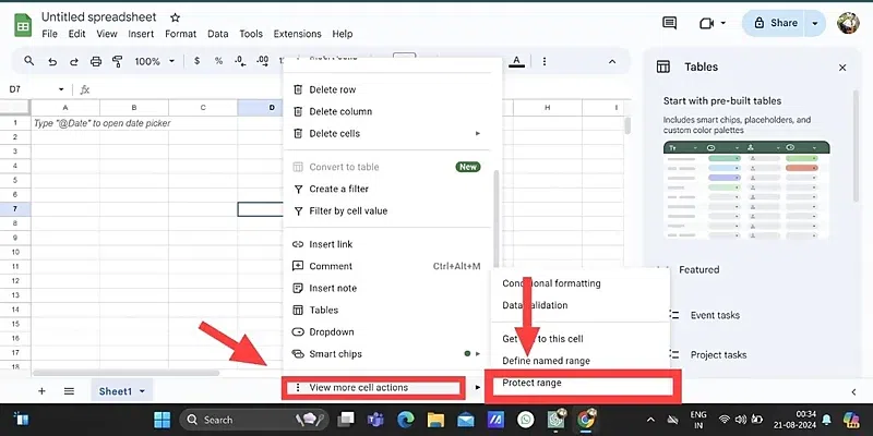
Hover Over "View More Cell Actions"

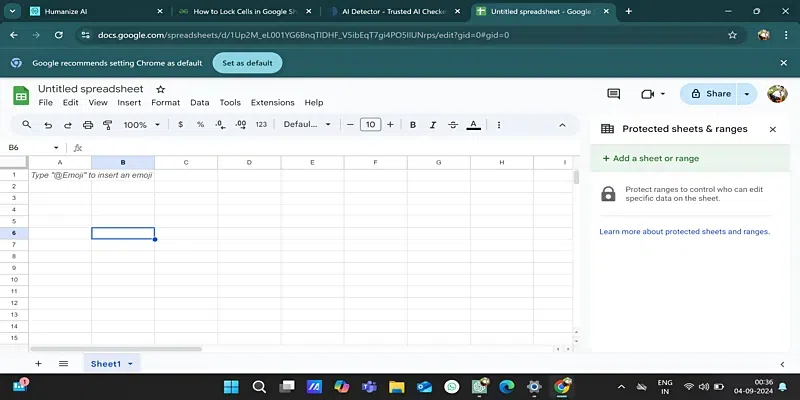
Step 3: Click on "Protect Range"

Click "Protect range" from the dropdown menu. This opens a side panel for range protection settings.

Click on "Protect Range"

Step 4: Click on "Add a Sheet or Range"

In the opened side panel, click "Add a sheet or range." This lets you identify the cells or a range to lock.

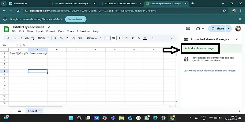
Click "Add a Sheet or Range"

Step 5: Define the Range or Cells to Lock

Mention the respective cell or range references you want to protect, or select those cells from your sheet directly. Also you can name the cell according to you.

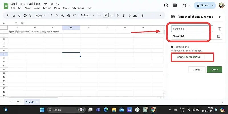
Select Which Cells You Want to Lock

Step 6: Click "Set Permissions"

Once you have selected the range, click "Set permissions." This will allow you to set who is authorized to modify these cells.

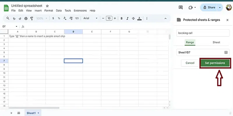
Click "Set Permissions"

Step 7: Adjust Permissions and Click "Done"

Choose who can edit the range from the options available—such as restricting it to specific people or only allowing certain changes—and then click "Done." Your selected cells are now locked from editing by unauthorized users.

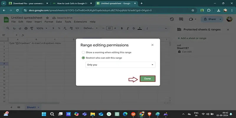
Click "Done"

2. How to Lock Google Sheets Formulas

Locking cells that contain formulas can prevent accidental edits that could disrupt your data calculations. Here’s how to do it:

Step 1: Select the Cells with Formulas

Highlight the cells containing the formulas you want to protect.

Right-click the Selected Cells

Step 2: Hover "View More Cell Actions"

Hover the mouse over the option to display "View more cell actions."

Hover "View More Cell Actions"

Step 3: Click "Protect Range"

Once "Protect range" is clicked, a protection side bar will pop up for the range.

Click "Protect Range"

Step 4: Click "Add a Sheet or Range" from the Side Panel

Click "Add a sheet or range" on the right-hand side panel to indicate which cells you want to lock.

Click "Add a Sheet or Range"

Step 5: Select Cells to Lock

Select the range of cells you want to lock, typing cell references or selecting cells directly on the worksheet. Also you can Name the cell according to you.

Select Cells to Lock

Step 6: Click "Set Permissions"

Click "Set permissions" to define who should have permissions to edit the locked cells.

Click "Set Permissions"

Step 7: Click "Custom"

Under the permission setting options, select the "Custom" option to allow setting editors for the locked cells.

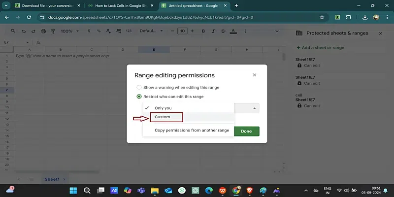
Click "Custom"

Step 8: Allow Editors to the Cells

Add the email addresses of users who need to have editing rights over the locked cells. Only these users will be able to make changes.

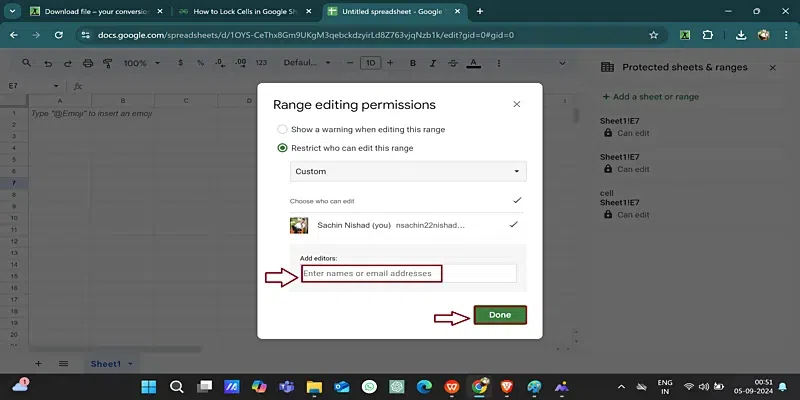
Allow Editors to the Cells

Then after all click on the **DONE.

3. How to Lock an Entire Sheet

Sometimes, you would want to lock the entire sheet so that there is no amendment. You do this by similar settings like locking individual cells, but this time the application is for the whole sheet. First, click on the sheet tab at the bottom of the page, then proceed with the same process outlined above concerning setting permissions and assigning editors.

4. How to Lock Cells in Google Sheets Shortcut

If you frequently work with Google Sheets and want a faster way to lock cells, using keyboard shortcuts can streamline your workflow. Here’s how to lock cells in Google Sheets using shortcuts:

Step 1: Select the Range of Cells

Highlight the cells you want to lock by clicking and dragging your mouse, or by using Shift + Arrow keys for quick selection.

Use the shortcut Alt + D on Windows or Option + D on Mac to quickly access the Data menu.

Step 3: Navigate to “Protected Sheets and Ranges”

Press the shortcut Alt + R to open the “Protected sheets and ranges” sidebar.

Step 4: Protect the Range

Click “Add a range or sheet” in the sidebar. Enter a description if necessary, and click “Set permissions.”

Step 5: Set Your Permissions

Use the provided options to choose who can edit the locked cells, then click “Done.”

Using these shortcuts not only saves time but also makes protecting your data more efficient. By mastering these steps, you’ll quickly secure your sheets against unwanted edits, keeping your work intact and organized.