Window Functions in SQL (original) (raw)
SQL window functions are essential for advanced data analysis and database management. They enable calculations across a specific set of rows, known as a “window,” while retaining the individual rows in the dataset. Unlike traditional **aggregate functions that summarize data for the entire group, window functions allow detailed calculations for specific partitions or **subsets of data.
This article provides a detailed explanation of **SQL window functions, including the **OVER clause, **partitioning, **ordering, and practical use cases, complete with outputs to help us understand their behavior.
What is a Window Function in SQL?
A **window function in SQL is a type of function that allows us to perform **calculations across a specific set of rows related to the current row. These calculations happen within a defined **window of data, and they are particularly useful for **aggregates, **rankings, and **cumulative totals without altering the dataset.
The OVER clause is key to defining this window. It partitions the data into different sets (using the **PARTITION BY clause) and orders them (using the **ORDER BY clause). These windows enable functions like **SUM(), **AVG(), **ROW_NUMBER(), **RANK(), and **DENSE_RANK() to be applied in a sophisticated manner.
**Syntax
SELECT column_name1,
window_function(column_name2)
OVER([PARTITION BY column_name1] [ORDER BY column_name3]) AS new_column
FROM table_name;
**Key Terms
- **window_function= any aggregate or ranking function
- **column_name1= column to be selected
- **column_name2= column on which window function is to be applied
- **column_name3= column on whose basis partition of rows is to be done
- **new_column= Name of new column
- **table_name= Name of table
**Types of Window Functions in SQL
SQL window functions can be categorized into two primary types: **aggregate window functions and **ranking window functions. These two types serve different purposes but share a common ability to perform calculations over a defined set of rows while retaining the original data.
The **employee table contains details about employees, such as their name, age, department, and salary.
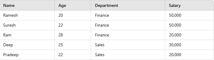
employees Table
**1. Aggregate Window Function
Aggregate window functions calculate aggregates over a window of rows while retaining individual rows. Common aggregate functions include:
- **SUM(): Sums values within a window.
- **AVG(): Calculates the average value within a window.
- **COUNT(): Counts the rows within a window.
- **MAX(): Returns the maximum value in the window.
- **MIN(): Returns the minimum value in the window.
**Example: Using AVG() to Calculate the Average Salary within each department:
SELECT Name, Age, Department, Salary,
AVG(Salary) OVER( PARTITION BY Department) AS Avg_Salary
FROM employee
**Output
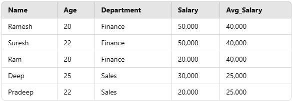
AVG() Function Example
**Explanation:
- The **AVG() function calculates the average salary for each department using the **PARTITION BY Department clause.
- The average salary is repeated for all rows in the respective department.
**2. Ranking Window Functions
These functions provide rankings of rows within a partition based on specific criteria. Common ranking functions include:
- **RANK(): Assigns ranks to rows, skipping ranks for duplicates.
- **DENSE_RANK(): Assigns ranks to rows without skipping rank numbers for duplicates.
- **ROW_NUMBER(): Assigns a unique number to each row in the result set.
**RANK() Function
The RANK() function assigns ranks to rows within a partition, with the same rank given to rows with identical values. If two rows share the same rank, the next rank is skipped.
Example: Using RANK() to Rank Employees by Salary
SELECT Name, Department, Salary,
RANK() OVER(PARTITION BY Department ORDER BY Salary DESC) AS emp_rank
FROM employee;
**Output
![]()
Rank Function Example
**Explanation:
Rows with the same salary (e.g., Ramesh and Suresh) are assigned the same rank. The next rank is skipped (e.g., rank 2) due to duplicate ranks.
**DENSE_RANK() Function
It assigns rank to each row within partition. Just like rank function first row is assigned rank 1 and rows having same value have same rank. The difference between RANK() and DENSE_RANK() is that in DENSE_RANK(), for the next rank after two same rank, consecutive integer is used, no rank is skipped.
Example:
SELECT Name, Department, Salary,
DENSE_RANK() OVER(PARTITION BY Department ORDER BY Salary DESC) AS emp_dense_rank
FROM employee;
**Output
| Name | Department | Salary | emp_dense_rank |
|---|---|---|---|
| Ramesh | Finance | 50,000 | 1 |
| Suresh | Finance | 50,000 | 1 |
| Ram | Finance | 20,000 | 2 |
| Deep | Sales | 30,000 | 1 |
| Pradeep | Sales | 20,000 | 2 |
**Explanation: The DENSE_RANK() function works similarly to RANK(), but it doesn’t skip rank numbers when there are ties. For example, if two employees have the same salary, both will receive rank 1, and the next employee will receive rank 2.
**ROW_NUMBER() Function
ROW_NUMBER() gives each row a unique number. It numbers rows from one to the total rows. The rows are put into **groups based on their values. Each group is called a **partition. In each partition, rows get numbers one after another. No two rows have the same number in a partition.
**Example: Using ROW_NUMBER() for Unique Row Numbers
SELECT Name, Department, Salary,
ROW_NUMBER() OVER(PARTITION BY Department ORDER BY Salary DESC) AS emp_row_no
FROM employee;
**Output
| Name | Department | Salary | emp_row_no |
|---|---|---|---|
| Ramesh | Finance | 50,000 | 1 |
| Suresh | Finance | 50,000 | 2 |
| Ram | Finance | 20,000 | 3 |
| Deep | Sales | 30,000 | 1 |
| Pradeep | Sales | 20,000 | 2 |
**Explanation: ROW_NUMBER() assigns a unique number to each employee based on their salary within the department. No two rows will have the same row number.
**Practical Use Cases for Window Functions
Window functions are extremely versatile and can be used in a variety of practical scenarios. Below are some examples of how these functions can be applied in real-world data analysis.
Example 1: Calculating Running Totals
We want to calculate a running total of sales for each day without resetting the total every time a new day starts.
SELECT Date, Sales,
SUM(Sales) OVER(ORDER BY Date) AS Running_Total
FROM sales_data;
**Explanation: This query calculates the cumulative total of sales for each day, ordered by date.
Example 2: Finding Top N Values in Each Category
We need to retrieve the top 3 employees in each department based on their salary.
WITH RankedEmployees AS (
SELECT Name, Department, Salary,
RANK() OVER(PARTITION BY Department ORDER BY Salary DESC) AS emp_rank
FROM employee
)
SELECT Name, Department, Salary
FROM RankedEmployees
WHERE emp_rank <= 3;
**Explanation: This query retrieves the top 3 employees per department based on salary. It uses RANK() to rank employees within each department and filters for the top 3
**Troubleshooting Common Issues with Window Functions
While SQL window functions are incredibly powerful, there are some common pitfalls and challenges that users may encounter:
- **Partitioning Error: Ensure that the
PARTITION BYclause is used correctly. If no partition is defined, the entire result set is treated as a single window. - **ORDER BY Within the Window: The
ORDER BYclause within the window function determines the order of calculations. Always verify that it aligns with the logic of your calculation. - **Performance Considerations: Window functions can be computationally expensive, especially on large datasets. Always ensure that your window functions are optimized and, if necessary, combined with appropriate indexes.
Conclusion
SQL **window functions are a crucial feature for advanced data analysis and provide flexibility when working with partitioned data. By mastering the **OVER clause, PARTITION BY, and ORDER BY, we can perform complex calculations like **aggregate calculations, **ranking, and **cumulative totals while preserving the row-level data. Using these **window functions SQL features, we can perform advanced data analysis tasks with ease. The combination of window functions with **ORDER BY and **PARTITION BY provides a flexible approach for data manipulation across **different types of datasets.