Zomato Data Analysis Using Python (original) (raw)

Last Updated : 17 Jan, 2025

Python and its following libraries are used to analyze Zomato data.

1. Numpy- With Numpy arrays, complex computations are executed quickly, and large calculations are handled efficiently.
2. Matplotlib- It has a wide range of features for creating high-quality plots, charts, histograms, scatter plots, and more.
3. Pandas- The library simplifies the loading of data frames into 2D arrays and provides functions for performing multiple analysis tasks in a single operation.
4. Seaborn- It offers a high-level interface for creating visually appealing and informative statistical graphics.

You can use Google Colab Notebook or Jupyter Notebook to simplify your task.

To address our analysis, we need to respond to the subsequent inquiries:

1. Do a greater number of restaurants provide online delivery as opposed to offline services?
2. Which types of restaurants are the most favored by the general public?
3. What price range is preferred by couples for their dinner at restaurants?

Before commencing the data analysis, the following steps are followed.

Following steps are followed before starting to analyze the data.

Step 1: Import necessary Python libraries.

Python `

import pandas as pd import numpy as np import matplotlib.pyplot as plt import seaborn as sns

`

Step 2: Create the data frame.

You can find the dataset link at the end of the article.

Python `

dataframe = pd.read_csv("Zomato data .csv") print(dataframe.head())

`

**Output:

                name online_order book_table   rate  votes  \  

0 Jalsa Yes Yes 4.1/5 775
1 Spice Elephant Yes No 4.1/5 787
2 San Churro Cafe Yes No 3.8/5 918
3 Addhuri Udupi Bhojana No No 3.7/5 88
4 Grand Village No No 3.8/5 166

approx_cost(for two people) listed_in(type)
0 800 Buffet
1 800 Buffet
2 800 Buffet
3 300 Buffet
4 600 Buffet

Before proceeding, let's convert the data type of the "rate" column to float and remove the denominator.

Python `

def handleRate(value): value=str(value).split('/') value=value[0]; return float(value)

dataframe['rate']=dataframe['rate'].apply(handleRate) print(dataframe.head())

`

**Output:

                name online_order book_table  rate  votes  \  

0 Jalsa Yes Yes 4.1 775
1 Spice Elephant Yes No 4.1 787
2 San Churro Cafe Yes No 3.8 918
3 Addhuri Udupi Bhojana No No 3.7 88
4 Grand Village No No 3.8 166

approx_cost(for two people) listed_in(type)
0 800 Buffet
1 800 Buffet
2 800 Buffet
3 300 Buffet
4 600 Buffet

To obtain a summary of the data frame, you can use the following code:-

Python `

dataframe.info()

`

**Output:

<class 'pandas.core.frame.DataFrame'>
RangeIndex: 148 entries, 0 to 147
Data columns (total 7 columns):

Column Non-Null Count Dtype

0 name 148 non-null object
1 online_order 148 non-null object
2 book_table 148 non-null object
3 rate 148 non-null float64
4 votes 148 non-null int64
5 approx_cost(for two people) 148 non-null int64
6 listed_in(type) 148 non-null object
dtypes: float64(1), int64(2), object(4)
memory usage: 8.2+ KB

We will now examine the data frame for the presence of any null values. This stage scans each column to see whether there are any missing values or empty cells. This allows us to detect any potential data gaps that must be addressed.

There is no NULL value in dataframe.

Let's explore the listed_in (type) column.

Python `

sns.countplot(x=dataframe['listed_in(type)']) plt.xlabel("Type of restaurant")

`

**Output:

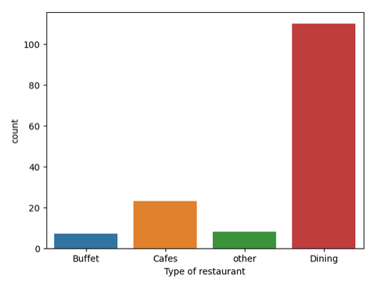
**Conclusion: The majority of the restaurants fall into the dining category.

Python `

grouped_data = dataframe.groupby('listed_in(type)')['votes'].sum() result = pd.DataFrame({'votes': grouped_data}) plt.plot(result, c='green', marker='o') plt.xlabel('Type of restaurant', c='red', size=20) plt.ylabel('Votes', c='red', size=20)

`

**Output:

Text(0, 0.5, 'Votes')

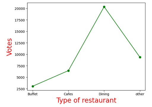
**Conclusion: Dining restaurants are preferred by a larger number of individuals.

Now we will determine the restaurant's name that received the maximum votes based on a given dataframe.

Python `

max_votes = dataframe['votes'].max() restaurant_with_max_votes = dataframe.loc[dataframe['votes'] == max_votes, 'name']

print('Restaurant(s) with the maximum votes:') print(restaurant_with_max_votes)

`

**Output:

Restaurant(s) with the maximum votes:
38 Empire Restaurant
Name: name, dtype: object

Let's explore the online_order column.

Python `

sns.countplot(x=dataframe['online_order'])

`

**Output:

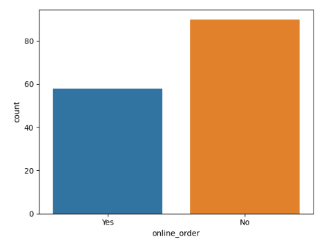
**Conclusion: This suggests that a majority of the restaurants do not accept online orders.

Let's explore the rate column.

Python `

plt.hist(dataframe['rate'],bins=5) plt.title('Ratings Distribution') plt.show()

`

**Output:

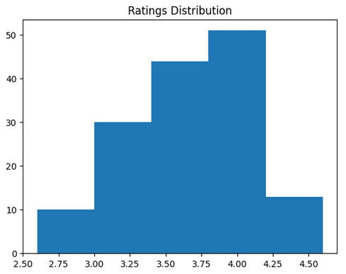
**Conclusion: The majority of restaurants received ratings ranging from 3.5 to 4.

Let's explore the approx_cost(for two people) column.

Python `

couple_data=dataframe['approx_cost(for two people)'] sns.countplot(x=couple_data)

`

**Output:

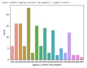
**Conclusion: The majority of couples prefer restaurants with an approximate cost of 300 rupees.

Now we will examine whether online orders receive higher ratings than offline orders.

Python `

plt.figure(figsize = (6,6)) sns.boxplot(x = 'online_order', y = 'rate', data = dataframe)

`

**Output:

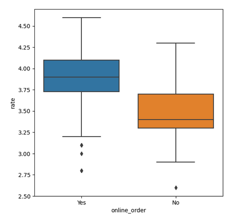
**CONCLUSION: Offline orders received lower ratings in comparison to online orders, which obtained excellent ratings.

Python `

pivot_table = dataframe.pivot_table(index='listed_in(type)', columns='online_order', aggfunc='size', fill_value=0) sns.heatmap(pivot_table, annot=True, cmap='YlGnBu', fmt='d') plt.title('Heatmap') plt.xlabel('Online Order') plt.ylabel('Listed In (Type)') plt.show()

`

**Output:

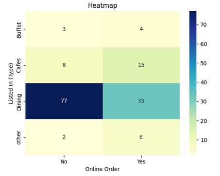
**CONCLUSION: Dining restaurants primarily accept offline orders, whereas cafes primarily receive online orders. This suggests that clients prefer to place orders in person at restaurants, but prefer online ordering at cafes.

You can download the data and source code from here:

• **Dataset: Zomato Data Set
• **Source Code: Zomato Data Analysis