Linear Response Surface with Strategy Single Stage (original) (raw)
Working Directory and Extraction of necessary files
- Create a working directory in the desired location to keep the LS-OPT project file and input files, as well as the LS-OPT program output, e.g. crash_linear_single.
- Extract all the files for the Single Stage from download section into the working directory.
Project Details
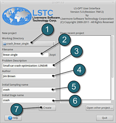
- Select the Working Directory of the LS-OPT project.
- Select a suitable name for the file under Filename (e.g. linear.single). The extension .lsopt is appended by LS-OPT.
- Description of the main task can e.g. be a suitable name for Problem Description ( in this case, Small car crash optimization: LINEAR , optional) .
- Input the name of the Author (optional).
- Choose a suitable name under the Initial Sampling name (e.g. crash).
- Choose a suitable name under the Initial Stage name (e.g. crash).
- Press the Create button to initiate the formation of the input file.
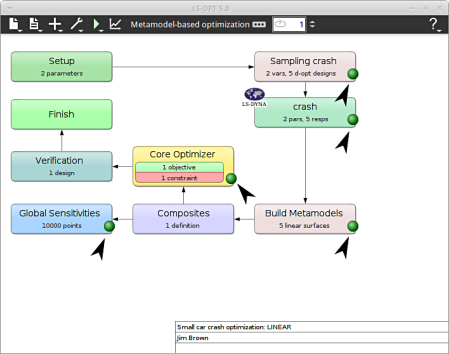
- The main GUI window of LS-OPT opens.
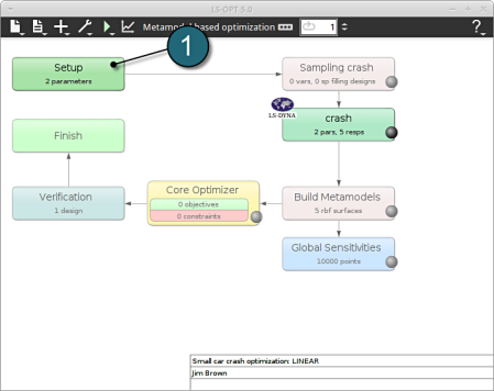
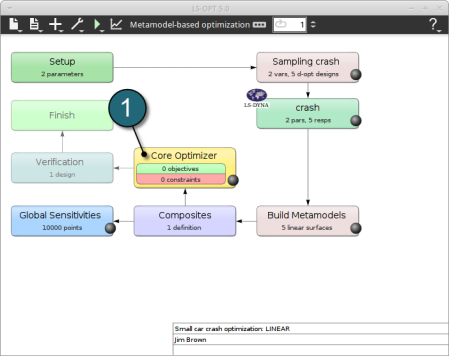
Home Screen Process Flowchart
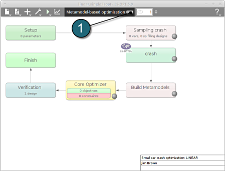
- Select the Task icon.
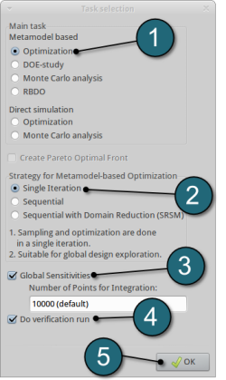
A window Task selection shall open.
Define the Main Task
- Select theradio button Optimization for the selection of the task
- The selection of the strategy for the metamodel is made to Single Iteration.
- To study Global Sensitivities for the input parameters remember to select the tick-box.
- The user has a choice to Do verification run by selecting the option. This will run an additional simulation using the optimal parameter values found on the metamodel to check the quality of the result.
- Click on the OK button to proceed.
- Setup
- Parameters
- Responses
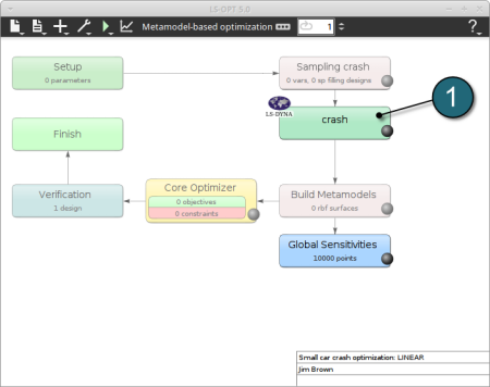
Home Screen Process Flowchart
- Double click on the crash box.
A window Stage crash shall open.
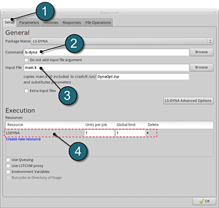
Define Input File Name and Command
- Select the Setup tab.
- For Command specify the LS-DYNA executable ls-dyna (This name can be different on your computer). On Windows, the command has to be specified using the absolute path.
- For Input File browse the parameterized file main.k. Parameters in LS-DYNA input files can be defined using *PARAMETER or the LS-OPT parameter format <<>>.
- For efficient usage of the computing power from the machine, choice on handling number of concurrent jobs can be made suitably in this section. (E.g., if the machine has 4CPUs, and to run each job on a single CPU : Units per job = 1, Global limit = 4).
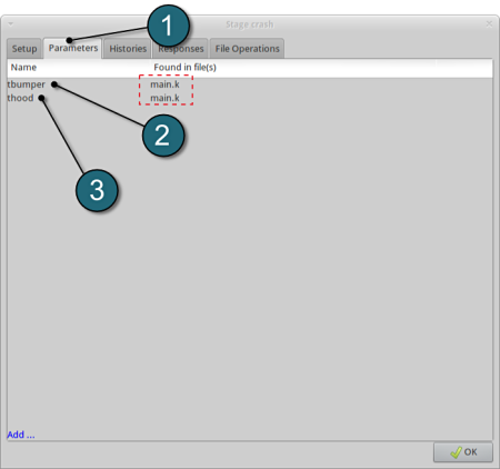
The parameters located in the selected Input File can be visualized in the adjoining tab Parameters.
Design Parameters.
- Select the Parameters tab.
- The first design parameter located in the input file main.k is displayed (In this case the thickness of the bumper, denoted as tbumper ).
- The second design parameter located in the input file main.k is displayed (In this case the thickness of the hood, denoted as thood ).
- The input file main.k is shown below for reference.
*KEYWORD *PARAMETER rtbumper,3.0,rthood,1.0 *INCLUDE ../../car5.k *END
Responses for Optimization
- The various responses for the optimization problem can be related to the car crash diagram shown below.


Fig. 1(a): Deformed vehicle after 50 msFig. 1(b): Design variables with part numbers
Add First Response
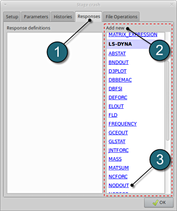
- Click on the Responses tab.
- Select the suitable response type from the various option available from the list under Add new.
- For the first response select the option NODOUT , which represents an interface to LS-DYNA nodout results. Note that LS-OPT reads the results from the binout database.
A separate window emerges named**; Edit response**. This enables the user to define the response in suitable steps.
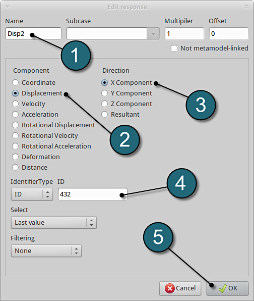
Define x-displacement of node 432
- For Response name enter Disp2.
- For Component select from the list Displacement.
- For Direction select X Component.
- For node ID enter 432.
- Click on the OK button to add the response.
- The Edit response tab closes and returns to the main page of the Responses tab in the Stage crash window.
Add Second Response
- To add an additional response select from the option NODOUT from the Add new on the Responses tab.
Define x-displacement of node 167
- To add the second response repeat in the similar manner for **Response nameDisp1 with node ID 167.
Add Third Response
- To add an additional response select from the option NODOUT from the Add new on the Responses tab.
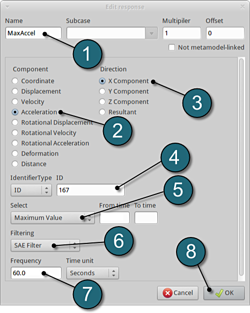
Define x-acceleration of node 167
- For Response name enter MaxAccel.
- For Component select from the list Acceleration.
- For Direction select X Component.
- For node ID enter 167.
- Select the Maximum Value option under Select. This will choose the max. value of acceleration in x-direction during the crash.
- For Filtering choose SAE Filter.
- Enter 60.0 for Frequency.
- Click on the OK button to add the response.
- The Edit response tab closes and returns to the main page of the Responses tab in the Stage crash window.
Add Fourth Response
- To add an additional response select from the option Injury from the Add new on the Responses tab.
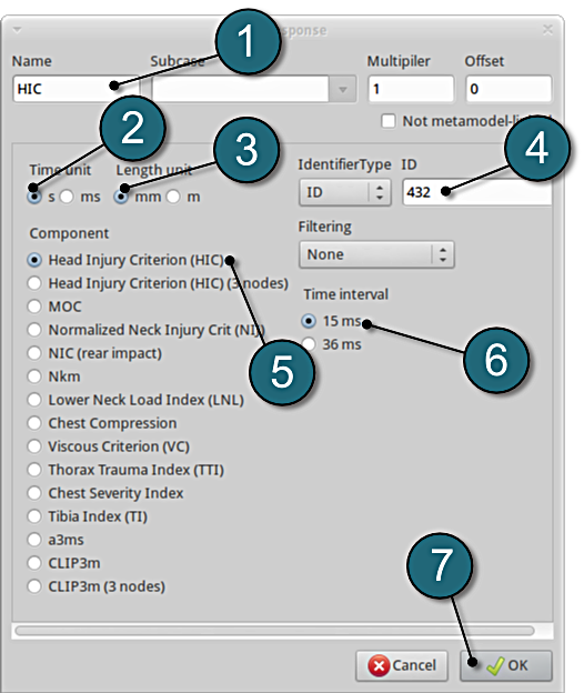
Define head injury coefficient of node 432
- For Response name enter HIC.
- For Time unit select s.
- For Length unit select mm.
- For Node ID enter 432.
- For Component select from the list Head Injury Criterion (HIC).
- For Time interval select 15 ms.
- Click on the OK button to add the response.
- The Edit response tab closes and returns to the main page of the Responses tab in the Stage crash window.
Add Fifth Response
- To add an additional response select from the option Mass from the Add new on the Responses tab.
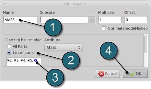
Define mass responses for structural components
- For Response name enter Mass.
- For Parts to be included select List of parts.
- In the empty box underneathenter 2. Push the add button (denoted as +) to add the various parts 3, 4 and 5.
- The part ID numbers can be found in Fig. 1 ( shown above ) bumper (2), hood (3), front (4) and underside (5).
- Click on the OK button to add the response.
- The Edit response tab closes and returns to the main page of the Responses tab in the Stage crash window.
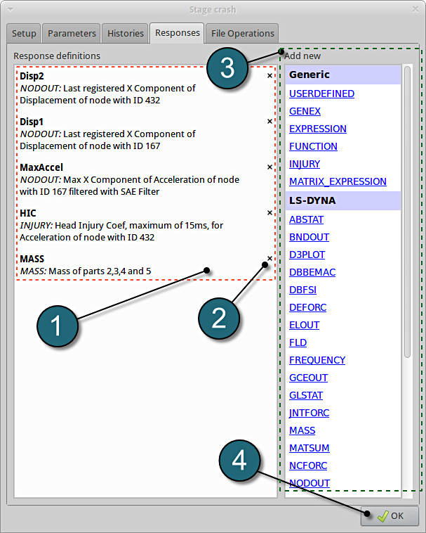
Responses Review
- The defined responses can be reviewed in the tab of the Response s under the Response definition. Necessary changes can be made by selecting the choice.
- To delete a Response definition click on the cross button (denoted as X).
- Additional responses can be added from the choice available under the Add new list as earlier.
- Click on the OK button to proceed.
- Parameter setup
- Stage Matrix
- Sampling Matrix
Home Screen Process Flowchart
- Double click on the Setup box.
A window Problem global setup shall open.
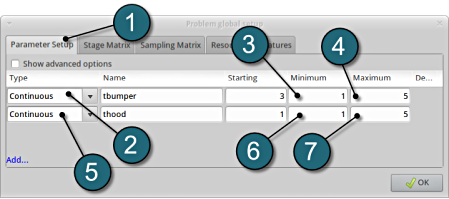
Define the Parameters.
- Select the Parameter Setup tab. Variables defined in Stages are automatically displayed here.
- For Type of tbumper switch the menu to Continuous.
- Enter 1 for the Minimum of the variable.
- Enter 5 for the Maximum of the variable.
- For Type of thood switch the menu to Continuous.
- Enter 1 for the Minimum of the variable.
- Enter 5 for the Maximum of the variable.
- The Starting values are read by LS-OPT automatically from the input file which includes them under the keyword *PARAMETER.
| Stage Matrix Select the Stage Matrix tab. You find a matrix of parameters vs. stages, and symbols that visualize if parameters are found in input files. |
|---|
| Sampling Matrix Select the Sampling Matrix tab.If you don't want to use a parameter as variable for a respective sampling, the variables can be switched off here. The parameters are treated as constants then. Click on the OK button to proceed_._ |
|---|
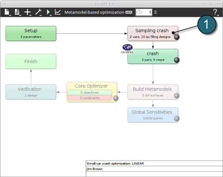
Home Screen Process Flowchart
- Double click on the Sampling crash box.
A window Sampling crash shall open.
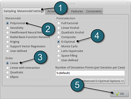
Define Metamodel Settings
- Select the Sampling Metamodel Settings tab.
- For Metamodel select from the list Polynomial.
- For Order of the Polynomial model we take Linear.
- Make sure that the Point Selection is set to D-Optimal, which is recommended.
- Click on the OK button to proceed.
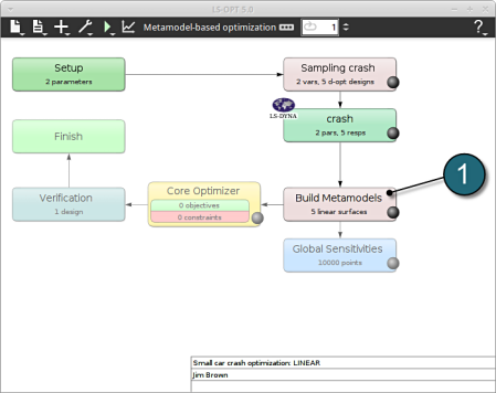
Build Metamodels
- To review the Metamodel properties for optimization, select the Build Metamodels box.
A window Sampling crash shall open which is the same as in the Sampling box. It's displayed twice in the main GUI to visualize the flowchart of the optimization process.
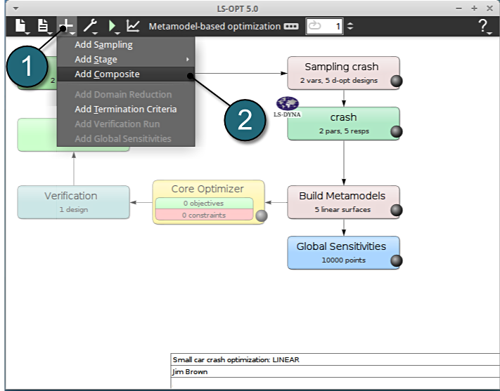
Home Screen Process Flowchart
- Click on the Add (denoted as +) located in the control bar.
- Select the option Add Composite from the list.
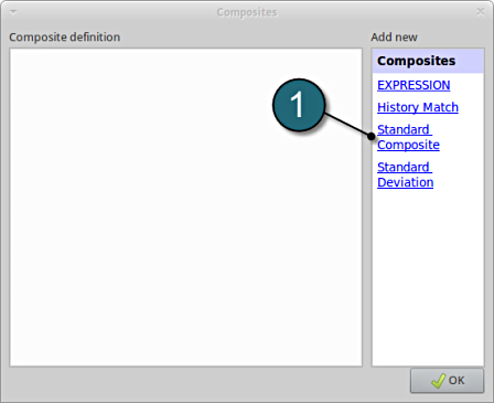
A window Composites shall open.
Composite Definition
- Select the option Standard Composite for the type of composite under the list for Add new.
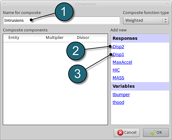
A separate window named as Composites shall open.
Add Composite
- Enter the Name for composite as Intrusions.
- Add Disp2 as the first component.
- Add Disp1 as the second component.
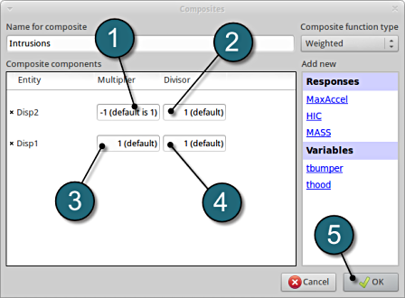
Define composite intrusion
- For Multiplier for Disp2 enter -1.
- Check for the Divisor for Disp2 at 1 (default).
- Check for the Multiplier for Disp1 at 1 (default).
- Check for the Divisor for Disp1 at 1 (default).
- Click on the OK button to proceed.
The composite is calculated as a weighted sum of the defined components, in this case
Intrusion = -Disp2+Disp1
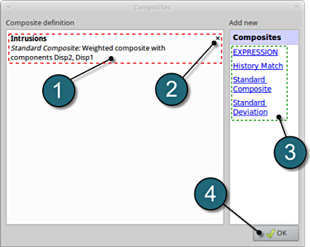
Composites Review
- The defined composite can be reviewed in the main page of the Composites under the Composite definition. Necessary changes can be made by selecting the choice.
- To delete a Composite definition click on the cross button (denoted as X).
- Additional Composite can be added from the choice available under the Add new list as earlier.
- Click on the OK button to proceed.
- Objectives
- Constraints
- Algorithms
Home Screen Process Flowchart
- Double click on the Optimization box.
A window Algorithms shall open.
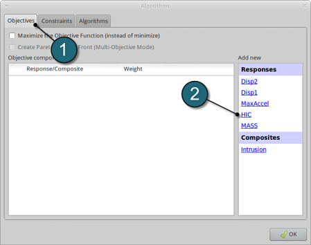
Add Objective
- Select the Objectives tab.
- From Response select HIC as the objective.
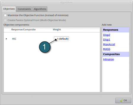
Define Objective
- For Weight leave the default 1. If you have several objective functions, you may assign weight to each one according to their importance.
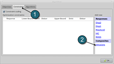
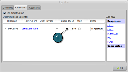
Add Constraints.
- Select the Constraints tab.
- From Composites select Intrusion s as the Optimization constraints.
Set bounds for Constraints.
- Select Set Upper Bound and enter 550.
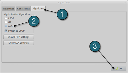
Optimization Algorithm.
- Select the Algorithms tab. Here, the algorithm used for the optimization on the metamodel can be selected.
- Make sure that the radio button for Adaptive Simulated Annealing (ASA) is selected and Switch to LFOP is checked. These are the default settings.
- Click on the OK button to proceed.
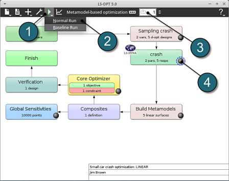
Run LS-Opt
- Click on the Run button from the Control Bar.
- Select Normal Run for execution.
- The user can get information on the current iteration during execution.
- At every stage the user has an option to view the progress of the program execution by selecting the LED on the crash tab.
- As seperate window Progress opens up.
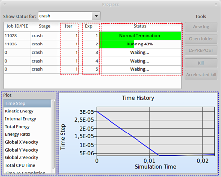
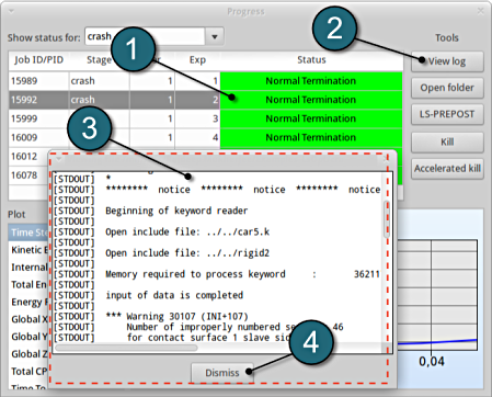
Progress
- The progress bar gives information on the status and several other details of the optimization progress.
- Underneath the status, the user has the option to view various plots of the computed values during execution vs the simulation time.
View Log
- Select the simulaiton point for which the log file is desired.
- Click on the View log button.
- A new window open containg the solver output, in this case the LS-DYNA output.
- Click on the Dismiss button to close the window and proceed.
- To view the status of the program during execution, observe the grey LED's at every stage of the process flow. Succesful completion of every stage is marked by turning respective LED green.
After completion of the program execution the user can view the results.
- Surface
- Computed vs. Predicted
- Accuracy
- Sensitivities
We can plot the response surface of the metamodel we've built. For example, we want to see the effect of the constraint on the optimization solution with respect to the variables thood and tbumper, do it as following:
Home Screen Process Flowchart
- The results can be viewed by selecting the view button on the task bar. A seperate window of LS-OPT Viewer opens up.
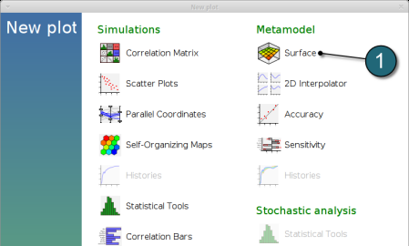
LS-OPT Viewer
- Select under Metamodel the item Surface.

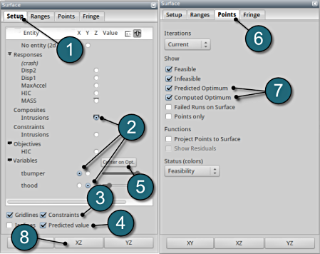
Constraints
- Select the Setup tab.
- Set the plot coordinates,
- Composites, Intrusions : z-coordinate
- Variables, tbumper : x-coordinate
- Variables,thood : y-coordinate.
- Pick Constraints to visualize feasible and infeasible regions on the metamodel, respectively.
- green : feasible region
- red : infeasible region.
- Choose Predicted value, a cross (+) appears on the surface.
- Click Center on Opt. to locate the cross at the optimal point.
- Select the Points tab.
- Pick Predicted Optimum and Computed Optimum.
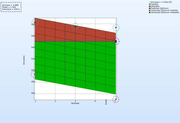
- To view the optimization constraints, we take a 2-D plot of Intrusions vs tbumber (variable).
Plot
- The 2-D plot clearly shows that the points in the red region ( intusions > 550 mm ) form the infeasible solutions, whereas the green points are the feasible solutions.
- The optimum point lies at the periphery of the feasible and infeasible domain. The predicted optimum point values are shown at the top-left corner of the plot.
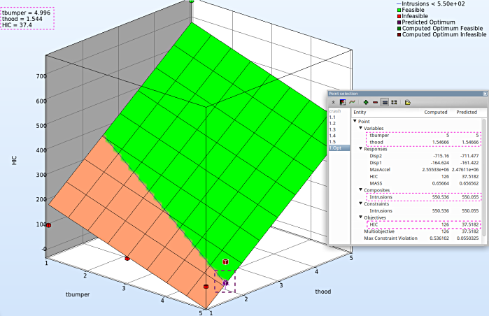
Objective - HIC Plot
- The primary objective of the optimization is to minmize the HIC.
- Repeat similar steps as the previous plot except for Z-axis select the Objective - HIC.
- Avoid Step. 8, to visulaize in a 3-D plot.
- It is important to note, the optimum is located at the lowest HIC in the feasible region.
- The user has the option to view the various entities by selecting any given point in the plot ( in this case the predicted optimum ). A point selection window opens up.
Study the change in each of the variables/responses and the accuracy of the predicted compared to the computed result.
The accuracy of the starting point and the approximate optimum points after the first iteration can be illustrated, e.g. for the response HIC you may find:
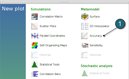
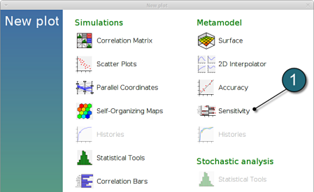
New Plot
- To view a new plot select the plot botton on the task bar. A seperate window of LS-OPT Viewer opens up.
LS-OPT Viewer
- Select under Optimization the item History.
- From the left side of the window select Responses → HIC.
- For Value to Plot select Value.
- If you want to see the accurate values, simply click nearby the red points. There appears a table, which states all the computed and predicted data, e.g. computed HIC vs. predicted HIC.
→ You can find out the appropriate values for the predicted (black) and the computed (red points) results. More iterations may lead to a better predictive capability.
→ A quality analysis is expected when the predicted (black line) and the computed (red points) are in close proximity.
(Note the range of the values when assessing the accuracy)
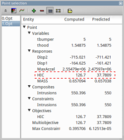
Predicted results compared to the computed result.
The user can select the respective points and compare the predicted values to the computed results for every iteration :
| Start ( 0.Opt ) | First Iteration ( 1.Opt ) | |||
|---|---|---|---|---|
| Predicted | Computed | Predicted | Computed | |
| thood | 1 | 1.549 | ||
| tbumper | 3 | 5 | ||
| MASS | 0.4103 | 0.4103 | 0.657 | 0.6571 |
| Intrusion | 577.3 | 575.7 | 550 | 550.4 |
| HIC | 74.64 | 68.02 | 37.78 | 126.7 |
| Max. Constr. Violation | 27.28 | 25.69 | 9.919e-5 | 0.3957 |
What is the approximation error of the result?
The approximation error indicators (predict the metamodel accuracy of the results) can be visualized in the LS-OPT Viewer.
New Plot
- To view a new plot select the plot button on the task bar. A seperate window of LS-OPT Viewer opens up.
LS-OPT Viewer
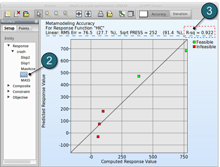
- Select under Metamodel the item Accuracy
- From Entity select Responses → HIC.
- We can find RMS Error and R2 (R-sq) above the plot.

→ Despite the coefficient of determination (R2) being high (=0.922), the RMS Error may need further improvement, e.g. more iterations or selection of a more suitable metamodel (e.g. Feedforward Neural Network or Radial Basis Function Network). Nevertheless for a raw estimate the result may be considered as acceptable.
→ It is important to note that the metamodel performs poor in cross-validation test using the SPRESS method. A relatively high SPRESS value (=91.4%) justifies a low confidence and a low predictive capability of the fitted metamodel.
- With the same procedure you may find the RMS Error, R² and SPRESS Residual of the other responses:
| | Mean Response Value | RMS Error | R2 | SPRESS Residual | | | ---------------------- | ---------- | ---------------- | --------------- | --------------- | | MASS | 0.7742 | 0 | 1 | 0 (0%) | | Disp1 | -159.3827 | 2.0309 (1.27%) | 0.4783 | 6.68 (4.19%) | | Disp2 | -694.5841 | 5.5486 (0.80%) | 0.9896 | 18.2 (2.62%) | | HIC | 275.726 | 76.5620 (27.74%) | 0.9225 | 252.11 (91.43%) |
Which variable appears to be the most important?
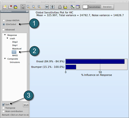
The significance of a variable for a response can be illustrated with ANOVA (analysis of variance) or GSA/Sobol (global sensitivity analysis), e.g for the response HIC you may find:
New Plot
- To view a new plot select the plot button on the task bar. A seperate window of LS-OPT Viewer opens up.
LS-OPT Viewer
ANOVA
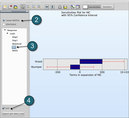
- Select under Metamodel select the item Sensitivity
- Select Linear ANOVA in the new window.
- From Response select HIC.
- Sort the variables according to their significance for HIC.
→ In this case the confidence intervals for both variables thood and tbumber are so wide (especially for tbumber) that one cannot end up with a conclusion about their linear significancies for the response HIC
GSA/Sobol
- Select GSA/Sobol.
- From Response select HIC.
- Sort the variables according to their significance for HIC.
→ We come to the same conclusion by using GSA. The influence of thood on HIC is 84.9%, larger than that of tbumper (15.1%).
GSA is a non-linear sensitivity measure, but evaluated on the metamodel, which is linear here. Hence it should lead to the same ranking than ANOVA.