Prediction of operons in microbial genomes (original) (raw)
Abstract
Operon structure is an important organization feature of bacterial genomes. Many sets of genes occur in the same order on multiple genomes; these conserved gene groupings represent candidate operons. This study describes a computational method to estimate the likelihood that such conserved gene sets form operons. The method was used to analyze 34 bacterial and archaeal genomes, and yielded more than 7600 pairs of genes that are highly likely (P ≥ 0.98) to belong to the same operon. The sensitivity of our method is 30–50% for the Escherichia coli genome. The predicted gene pairs are available from our World Wide Web site http://www.tigr.org/tigr-scripts/operons/operons.cgi.
INTRODUCTION
Many of the genes in bacterial genomes are organized into operons, which for the purposes of this paper will be defined as a series of genes that are transcribed into a single mRNA molecule. Co-transcribed genes often fill related roles in the function of the organism, sometimes binding to one another, or acting as part of the same metabolic pathway. In addition, co-transcribed genes are co-regulated at the transcriptional level. Identifying the genes that are grouped together into operons may enhance our knowledge of gene regulation and function, and such information is an important addition to genome annotation (1).
Computational algorithms to locate operons have been developed previously, primarily for Escherichia coli (2,3). Earlier methods were based on finding signals that occur on the boundaries of operons: transcription promoters on the 5′ end, and terminators on the 3′ end. Such approaches can only be effective for organisms whose promoters and terminators are well known, such as E.coli. Even so, the accuracy of such operon finding methods has been reported to be only ∼60% (3). One possible reason for the difficulty these methods have in making accurate predictions of operon structure is that promoter and terminator sequence motifs are not well characterized, even in E.coli. Making the problem even harder is the fact that operons sometimes include internal promoters and terminators (4–6). Another method (7) uses a combination of gene expression data, functional annotation and other experimental data, which is primarily applicable to well studied genomes such as E.coli. Finally, some methods rely on distances between adjacent genes and functional gene annotation (yielding ∼75% accuracy for operon predictions or 82% for gene pairs prediction) (8).
An alternative method to predict operons is based on finding gene clusters where gene order and orientation is conserved in two or more genomes (9–12). This approach does not rely on experimental data, but instead uses the genome sequence and gene locations. In this study, we describe a computational and statistical method that finds such conserved gene clusters and assigns to each one a probability that the cluster is an operon. We have identified over 7600 pairs of genes where the probability that the genes belong to the same operon is 0.98 or higher; that is, at least 98% of these gene pairs are expected to represent operons (or parts of operons). At this high level of specificity, the algorithm finds only ∼30–50% of the likely gene pairs, but the high specificity values make it possible to add them to computationally-assisted genome annotation.
Microbial genomes seem to undergo frequent rearrangements; even two strains of the same bacteria may have significant numbers of genes that are adjacent in one but not the other strain (e.g. 26% for Chlamydia pneumoniae strains CWL029 and AR39; 14% for Helicobacter pylori strains 26695 and J99). Some genes, however, tend to be located together in multiple genomes, including organisms as distantly related as archaea and bacteria. It would be expected that positive evolutionary selection for operons would result in similarly ordered sets of genes across phylogenetically-distant genomes. Alternatively, conservation of gene order between evolutionarily similar organisms may simply reflect the genes’ positions in the common ancestor.
How confident can we be that genes that are located in the same order in different genomes belong to the same operon? If a gene cluster is shared by a large number of genomes, then intuitively one would expect that the probability is very high that the cluster represents an operon. Only a small number of such stable gene clusters can be found across multiple genomes in the data available to date (13). A much greater number of clusters are shared by just two genomes. The question is whether one can assert with high probability that these gene clusters are in fact operons. In many cases, the answer is yes; below, we describe our method for estimating the probability that the conserved gene cluster represents an operon and we describe its results on 34 complete prokaryotic genomes.
MATERIALS AND METHODS
We will use the term ‘gene pair’ to refer to two adjacent genes separated by ≤200 bp. There are two types of gene pairs: genes of an S pair are on the same strand, and genes of a D pair are on different strands. Genes on different strands necessarily belong to different operons, while genes on the same strand may belong to the same operon (an SO pair) or to different operons (an SN pair). Some genes are transcribed and regulated separately from adjacent genes on either side; for simplicity, we may refer to these as one-gene operons.
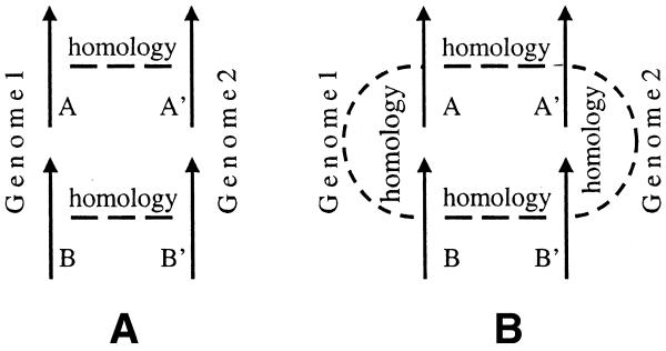
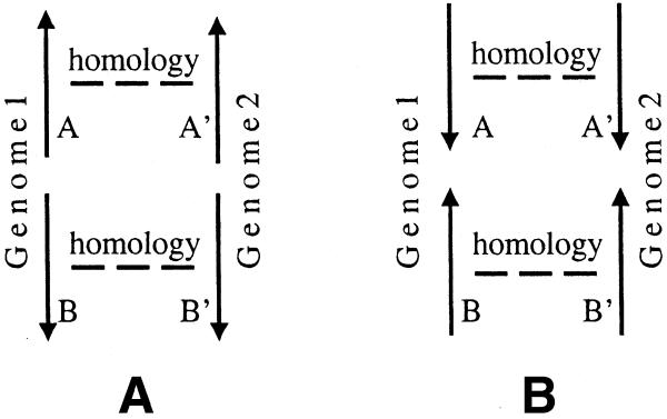
We searched all genes from 34 bacterial and archaeal genomes against one another using BLASTP (14,15), considering only genes with an E-value less than 10–5 as possible homologs. A conserved gene pair is defined as two adjacent genes (A,B) for which a homologous gene pair (A′,B′) can be found in another genome, such that A is homologous to A′, B is homologous to B′, and the pair (A′,B′) are adjacent (Figs 1A and 2). A pair is not considered conserved if the similarity between A and B is higher than the similarity between A and A′ or B and B′; this situation might be better explained as the result of independent recent duplications of one of the genes in each genome (Fig. 1B).
Figure 1.
(A) Conserved S gene pair. (B) A gene pair that has a higher similarity between its own genes than with a gene pair of the other genome is not considered to be conserved.
Figure 2.
Conserved D gene pairs.
Genes in conserved S pairs are candidates for membership in the same operon (SO pairs). Below we describe how to estimate the probability that genes in a conserved S pair belong to the same operon.
First, consider the case in which only two genomes are being compared, and conserved gene pairs have been identified between the two. Four different explanations (excluding independent gene duplication, which was explained above) can account for a conserved pair: (i) genes in the conserved pair belong to the same operon; (ii) genes in the conserved pair were inherited from a common ancestor and have maintained their adjacent locations; (iii) a lateral gene transfer event (16) moved the gene pair from one genome into the other; (iv) the conserved genes are adjacent by chance.
Genes within SN and D pairs (whether conserved or not) do not form operons; the only difference between these types is the orientation of the genes. The probability that common ancestry (ii above), lateral transfer (iii) or chance (iv) generated the conserved pair does not depend on the orientations of the genes and, therefore, the frequencies of such gene pairs should be the same between SN and D pairs:
P(conserved | SN) = P(conserved | D) 1
where P(conserved | x) is a probability that a gene pair of type x is conserved.
Next, let D, S, SN, SO represent the occurrence of gene pairs with type D, S, SN and SO, respectively. The term conserved will represent the event that a gene pair is conserved, and the notation (A,B) will indicate the joint occurrence of A and B. Applying the definition of conditional probability, P(B | A) = P(A,B)/P(A) to these events gives:
P(SN,(conserved,S)) = P(SN | (conserved,S)) × P(conserved,S) 2
and
P(SN,(conserved,S)) = P((conserved,S) | SN) × P(SN) 3
P(conserved,S) = P(conserved | S) × P(S) 4
P(SN,S) = P(SN | S) × P(S) 5
The SN gene pairs are a subset of S pairs; therefore, event S always occurs if SN occurs, which means that:
P(SN,S) = P(SN) 6
Therefore:
P((conserved,S) | SN) = P(conserved | SN) 7
Combining equations 2 to 7 gives:
 8
8
Combining equations 1 and 8 gives:
 9
9
In other words, if an S gene pair is conserved, then the probability that it has subtype SN scales by a factor that is equal to k:
 10
10
First we will calculate k and then P(SN | S).
P(conserved | D) is the probability that a type D gene pair from the first genome is conserved in the second genome, which is simply the number of conserved D pairs divided by the number of all D pairs:
 11
11
where N(x) is the number of gene pairs of the type x in the first genome.
P(conserved | S) is calculated similarly:
 12
12
Combining equations 10 to 12 gives an equation where all variables on the right can be easily calculated. The gene coordinates and directions provide information about S and D pairs, and BLASTP (15) finds conserved pairs:
 13
13
The value of k is relatively small for genomes that are not close relatives, corresponding to the intuitive notion that if a gene pair is conserved between distantly-related organisms, the probability that the genes belong to the same operon increases.
Although equation 11 uses the standard statistical definition of posterior probability, this estimate is not stable if the number of conserved D pairs, N(conserved | D), is close to zero, because small random variations in this value may significantly change the estimate of P(conserved | D). Figure 3 (gray line) shows the dependence of k on P(conserved). This function was constructed by calculating k values for every pair from all 34 genomes. In order to minimize the error produced by random variations in N(conserved | D), we approximated the dependence by a smoother curve (black line). The curve was obtained by dividing P(conserved) into small intervals and calculating the average k for each interval (k). This smoothed estimate was used only when N(conserved | D) was close to zero.
Figure 3.
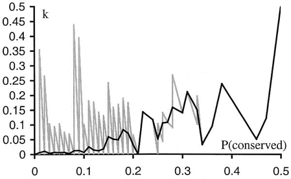
k – P(conserved) dependence (gray line) and its approximation k – P(conserved) (black line). The approximation was done by dividing the P(conserved) into intervals with length 0.01 and calculating average value of k on each interval.
In order to calculate P(SN | S) we have to evaluate the number of operons in the first genome. Let the term ‘directon’ indicate a maximal set of adjacent genes located on the same DNA strand; i.e. the adjacent genes on both the 5′ and 3′ sides of the directon fall on the opposite strand. In order to estimate the average number of operons in a directon, we made the assumption that the direction of an operon does not depend on the operons on either side of it. Due to insufficient experimental data, we cannot directly check if this assumption is true, but the number of operons in E.coli calculated using this assumption is consistent with other estimates, which are partly based on experimental data (3).
If we define a transcriptional unit containing just one gene as a single-gene operon, then every directon has at least one operon. The probability that a randomly chosen directon has exactly n operons is just the probability that operons 2 to n have the same direction as the first operon and that the next operon has a different direction. If orientation of operons is random, then this probability is ()n and the average number of operons in a directon is:
 14
14
The above summation reduces to m = 2, which means that the number of operons in the genome is twice the number of directons:
N(operons) = 2_N_(directons) 15
N(operons) is also the number of operon boundaries in the genome; that is, the sites where one operon ends and the next one begins.
Based on the available experimental data, genes that are separated by >200 bp almost always belong to different operons (3). Thus, almost all genes that are adjacent but do not form a gene pair (i.e. separated by ≥200 bp) have an operon boundary between them. Recall that our definition of pairs includes only adjacent genes at a distance ≤200 bp; ‘non-pairs’ in our notation refer to adjacent genes with distances >200 bp. By definition, the number of all genes is the sum of adjacent pairs plus adjacent non-pairs. The number of adjacent non-pairs is the number of all genes minus the number of gene pairs:
N(adjacent, non-pairs) = N(genes) – N(pairs) 16
Genes of D pairs also always belong to different operons. All the other operon boundaries are located in S pairs and the number of these remaining boundaries is equal to number of SN pairs in the genome:
N(SN pairs) = N(operons) – N(adjacent, non-pairs) – N(D pairs) 17
Combining equations 16 and 17 and considering that N(pairs) = N(D pairs) + N(S pairs) gives:
N(SN pairs) = 2_N_(directons) + N(S pairs) – N(genes) 18
P(SN | S) is the ratio of the number of SN pairs to the S pairs in the genome:
 19
19
We can now calculate the probability that the genes of a conserved S gene pair belong to the same operon:
P = (1 – P(SN | (conserved, S)) 20
Combining equations 9, 10, 19 and 20 gives the probability value:
 21
21
The calculation of k was described above, and all the other variables in the right hand side of the equation can easily be calculated from the coordinates and directions of the genes in the genome.
A gene pair may have homologous gene pairs in more than one other genome, in which case our calculation will assign multiple probabilities. In such cases, our algorithm assigns the highest probability value to the gene pair.
Thus far, we have considered the case when just two genomes were being compared. In order to find as many operons as possible, we compared each genome with all other completed genomes (34 at the time of this study). This approach, however, dramatically increases the probability of finding a conserved gene pair by chance; obviously when many more gene pairs are compared, the odds of a false positive increase.
Using D pairs, we can calculate the average number of random matches in gene pairs between two unrelated genomes, which turns out to be 0.1 or fewer. This chance probability should be the same for S pairs. Thus, for a given genome, the number of conserved S pairs that have homologs in a single unrelated genome due to chance alone should be, at most, 0.1_G_, where G is the number of other genomes in the database. The probability of a given conserved S pair to have a homolog due to chance is  and the probability to have homologs in h unrelated genomes is:
 22
22
Here, G is the number of all genomes in the database (excluding one genome with a given gene pair) and h is the number of those genomes where homologs for a given gene pair were found.
Thus, we need to adjust the probability value to account for the number of genomes in the database and the number of random homologous gene pairs that are expected for a given gene pair:

 23
23
For our database, in which G = 33, the factor 0.1_G_ is quite small and, even for the most common case where h = 1 (the chance gene pair occurs in just two genomes), the probability that the genes belong to the same operon will decrease by less than 0.01. However, as the database continues to grow, the value of P for gene pairs that are shared by only two genomes will decrease linearly with the number of genomes. For example, if the database has 1000 genomes, then the value of P for a gene pair that is shared by only two genomes will be about 0.7, which is much lower than any reasonable cutoff. At the same time, the number of homologs for the true SO gene pairs should grow with database size, and the estimated probability that the genes belong to the same operon will increase.
In the beginning of this section we made a few assumptions that allowed us to derive equation 23, and here we will discuss them in more detail. First, we assumed that there are four different factors that may result in conserved gene order: operons, common ancestor, lateral gene transfer and chance. However, we did not take into account the possibility that some gene clusters can be conserved due to two (or maybe even three) of these factors; i.e. we assume that if a gene cluster is conserved due to a common ancestor, it does not represent an operon. Thus, we overestimate P(SN | (conserved,S)), which results in underestimation of P in equations 20 and 23. A similar situation occurs with lateral gene transfer. A gene cluster can represent an operon and it can also have been recently transferred from one genome into another. Lawrence (17,18) suggested a theory that DNA fragments that represent operons are more likely to be successfully transferred from one taxon to another. This theory also suggests that lateral gene transfer is one of the mechanisms of operon formation. So, at least some lateral gene transfer events may represent operons and this may result in overestimation of P(SN | (conserved,S)) and underestimation of P.
There is also another important factor that may impact our results. In our work we assume that ‘D’ pairs never represent operons and therefore their order should not be conserved. However, co-regulation of divergently transcribed genes that share upstream regulatory elements can also lead to conservation of gene order. Such a mechanism of co-regulation was reported in yeast (19) and we cannot exclude the possibility that it might be present in bacteria. Thus, treating all D pairs as an estimate of the rate of SN pairs may lead to an overestimate of the rate of false positives and underestimation of P.
Based on the above considerations we rewrite equation 23 in the following form:

 24
24
RESULTS AND DISCUSSION
Using the algorithm described above, we found 7699 gene pairs in 34 bacterial genomes for which the probability that the genes belong to the same operon is ≥0.98. This means that at least 7545 (98%) of these pairs should represent true operons (or parts of operons). The next logical issue is how this compares to experimental data, for which one needs a set of confirmed operons on which to test the method.
Escherichia coli is the only organism for which a substantial number of experimentally-determined operons exist, and therefore we considered how many of these documented operons were found by our algorithm (our algorithm found 510 SO gene pairs with P ≥ 0.98 in E.coli). The two most complete sets of E.coli operons with experimental evidence are contained in RegulonDB (2; http://www.cifn.unam.mx/Computational_Biology/E.coli-predictions/) and CGSC DB (20; http://cgsc.biology.yale.edu/). The latter contains more recent data, but it is not consistent with the genome annotation used here (21), and mapping those operons to the genome is not always possible with the available data. We therefore used RegulonDB to construct the test set and used CGSC DB for additional information about particular operons.
RegulonDB contains 389 documented operons. It also contains many gene pairs that are documented as belonging to different operons; for example, genes A, B, C and D might be adjacent and on the same strand, and the documented operon might include only genes A, B and C. We interpreted this as an assertion that D does not belong to the operon; thus, AB and BC are SO gene pairs, whereas CD is an SN gene pair. In total, RegulonDB contains 541 SO gene pairs and 263 SN gene pairs.
For the test of the algorithm, a predicted SO gene pair is called a true positive if it corresponds to an SO gene pair from the testing set. A false positive is a predicted SO gene pair that is documented as an SN pair in the testing set. Here, we consider only 285 predictions that correspond to the gene pairs from the testing set. Specificity is the ratio of number of true positives to number of all positive predictions; i.e. it is an experimental analog of our _P_-value (multiplied by 100%). If all our assumptions are correct, the two values should be the same.
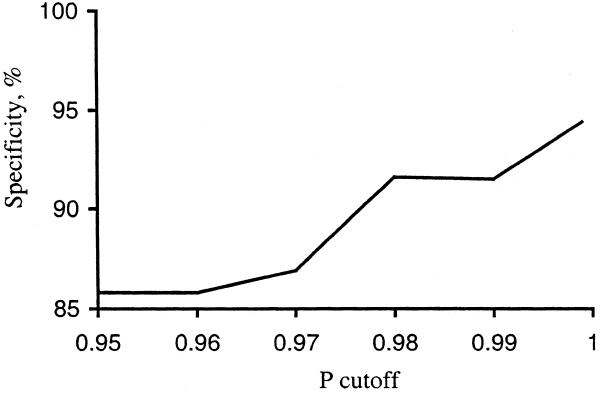
Figure 4 shows the relationship between specificity and P. The specificity obtained from experimental data is slightly lower than the _P_-value. With P ≥ 0.98 we would expect six (or fewer) false positives, but comparison with the RegulonDB (which is not a complete list of all E.coli operons) gives 24 false positives. Upon further investigation, we found that some of this difference may be caused by incorrect experimental data in RegulonDB. For example, we examined the 24 false positives with P ≥ 0.98 and found data from the CGSC database that indicated that at least 10 of these are in fact true positives. This can be explained by the fact that it is easier to detect (experimentally) co-transcription and co-regulation than it is to detect the absence of co-transcription. In fact, some genes appear to be co-transcribed only in special conditions. For example, Nakamura and Mizusawa (22) concluded that E.coli genes infB and rpsO belong to different operons, but a later experiment (23) showed that there is some transcriptional read-through between them, which functionally links these two suboperons into one complex system.
Figure 4.
Dependence of specificity on the P cutoff.
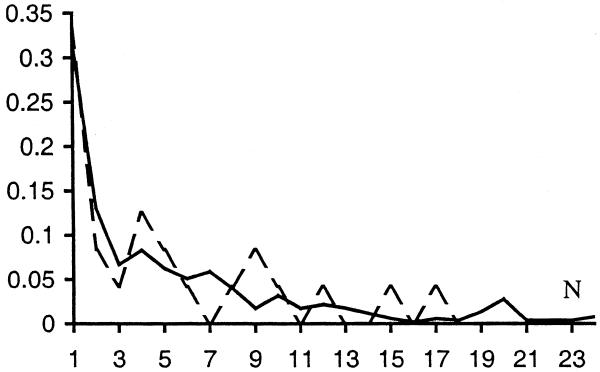
Many conserved S gene pairs have homologs in more than one genome in the current database. The normalized distribution of the number of such genomes for E.coli is indicated by a solid line in Figure 5. The dashed line shows the same distribution for the 24 false positives. The two distributions look similar, although the distribution for false positives is noisy because it is based on a small amount of data. Sixteen out of 24 false positives are shared by more than two genomes, six out of them are shared by at least four distantly-related genomes (as defined by ribosomal RNA phylogeny) and there is one false positive that is shared by 17 genomes (seven of these 16 gene pairs are the true positives confirmed by CGSC as mentioned above). Considering that all of the conserved D pairs for E.coli are shared by just two unrelated genomes each, it seems likely that some of the 16 gene pairs shared by more than two genomes are in fact true positives.
Figure 5.
Normalized distribution of N for conserved SO gene pairs in E.coli. N is the number of genomes with gene pairs homologous to the given E.coli gene pair. Solid line, all conserved pairs with P ≥ 0.98; dashed line, false positives.
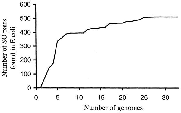
The final question is what percentage of true operons are found by this method, i.e. how sensitive is it? Although it is highly specific, it does not find nearly all the operons in a genome. It can only find those that are common to different genomes, and this is a function of the number of completely sequenced genomes and their evolutionary relationships. For the E.coli test set, ∼50% of the experimentally-determined gene pairs from the Regulon database are found by the algorithm. Of course, the experimentally-determined operons represent only a fraction of all E.coli operons. Our algorithm finds many operons for which there is no experimental evidence. Our estimation of sensitivity may be biased upward because conserved operons (i.e. those operons that the program can find) may be more likely to be studied experimentally than other operons. Using our own theoretical prediction of the expected number of operons in the E.coli genome will give an estimate of ∼30% sensitivity. In Figure 6, we show the results of running our method with fewer than 34 genomes; as shown, sensitivity increases as more genomes become available. However, this improvement in sensitivity may have a limit, because most genomes have some number of unique genes. We also note that our method is not designed to predict whole operons—it predicts pairs of genes that belong to the same operon (i.e. parts of operons). Sometimes the predicted gene pairs can be combined into longer units. For example, if genes A and B belong to the same operon with a probability _P_AB and genes B and C are a part of an operon with the probability _P_BC than the probability that genes A, B and C belong to the same operon can be calculated as _P_AB × _P_BC.
Figure 6.
Dependence of the number of predicted SO pairs in E.coli (with P ≥ 0.98) on the number of genomes to which E.coli was compared.
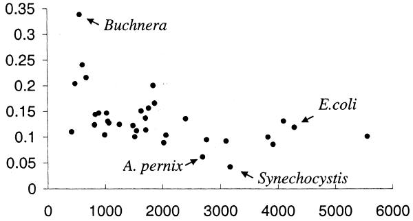
We do not have enough experimental data to estimate the sensitivity of our method for any genome other than E.coli, but we can compare the numbers of predicted gene pairs for different genomes. Figure 7 shows numbers of predicted gene pairs (with P ≥ 0.98) scaled by the number of genes in each of 34 genomes. There is a correlation between genome size and number of predicted gene pairs: smaller genomes have higher numbers of predicted gene pairs per gene. The most likely explanation of this fact is that smaller genomes have a higher percentage of genes common to different genomes. The only genome that significantly diverges from this pattern is the Buchnera genome (24), which has a much higher number of predicted gene pairs than other genomes of the same size. This might indicate that Buchnera has more or larger operons in its genome. Buchnera stands out as the only symbiotic bacteria in our set; all the others are either pathogens or free-living organisms.
Figure 7.
Number of predicted gene pairs (with P ≥ 0.98) in different bacterial and archaeal genomes. The _x_-axis shows number of genes in the genome and _y_-axis shows number of found gene pairs in these genomes scaled by number of genes.
The database of the predicted SO gene pairs is available on the Web at http://www.tigr.org/tigr-scripts/operons/operons.cgi.
Acknowledgments
ACKNOWLEDGEMENTS
The authors want to thank Michael Heaney and Susan Lo for database support, Jeremy Peterson for help in linking our data to other TIGR databases and Mary Berlyn for kindly providing us with a list of documented operons from the CGSC database. Thanks to the anonymous reviewers for thoughtful comments. This work was supported in part by NSF grant KDI-9980088 and NIH grant R01-LM06845 to S.L.S.
References
- 1.Hodgman T.C. (2000) A historical perspective on gene/protein functional assignment. Bioinformatics, 16, 10–15. [DOI] [PubMed] [Google Scholar]
- 2.Huerta A.M., Salgado,H., Thieffry,D. and Collado-Vides,J. (1998) RegulonDB: a database on transcriptional regulation in Escherichia coli. Nucleic Acids Res., 26, 55–59. [DOI] [PMC free article] [PubMed] [Google Scholar]
- 3.Yada T., Nakao,M., Totoki,Y. and Nakai,K. (1999) Modeling and predicting transcriptional units of Escherichia coli genes using hidden Markov models. Bioinformatics, 15, 987–993. [DOI] [PubMed] [Google Scholar]
- 4.Homuth G., Masuda,S., Mogk,A., Kobayashi,Y. and Schumann,W. (1997) The dnaK operon of Bacillus subtilis is heptacistronic. J. Bacteriol ., 179, 1153–1164. [DOI] [PMC free article] [PubMed] [Google Scholar]
- 5.Tsui H.C., Zhao,G., Feng,G., Leung,H.C. and Winkler,M.E. (1994) The mutL repair gene of Escherichia coli K-12 forms a superoperon with a gene encoding a new cell-wall amidase. Mol. Microbiol., 11, 189–202. [DOI] [PubMed] [Google Scholar]
- 6.Yanofsky C. (2000) Transcription attenuation: once viewed as a novel regulatory strategy. J. Bacteriol ., 182, 1–8. [DOI] [PMC free article] [PubMed] [Google Scholar]
- 7.Craven M., Page,D., Shavlik,J., Bockhorst,J. and Glasner,J. (2000) A probabilistic learning approach to whole-genome operon prediction. ISMB, 8, 116–127. [PubMed] [Google Scholar]
- 8.Salgado H., Moreno-Hagelsieb,G., Smith,T.F. and Collado-Vides,J. (2000) Operons in Escherichia coli: genomic analyses and predictions. Proc. Natl Acad. Sci. USA, 97, 6652–6657. [DOI] [PMC free article] [PubMed] [Google Scholar]
- 9.Siefert J.L., Martin,K.A., Abdi,F., Widger,W.R. and Fox,G.E. (1997) Conserved gene clusters in bacterial genomes provide further support for the primacy of RNA. J. Mol. Evol., 45, 467–472. [DOI] [PubMed] [Google Scholar]
- 10.Bansal A.K. (1999) An automated comparative analysis of 17 complete microbial genomes. Bioinformatics, 15, 900–908. [DOI] [PubMed] [Google Scholar]
- 11.Overbeek R., Fonstein,M., D’Souza,M., Pusch,G.D. and Maltsev,N. (1999) The use of gene clusters to infer functional coupling. Proc. Natl Acad. Sci. USA, 96, 2896–2901. [DOI] [PMC free article] [PubMed] [Google Scholar]
- 12.Huynen M., Snel,B., Lathe,W.,III and Bork,P. (2000) Exploitation of gene context. Curr. Opin. Struct. Biol., 10, 366–370. [DOI] [PubMed] [Google Scholar]
- 13.Itoh T., Takemoto,K., Mori,H. and Gojobori,T. (1999) Evolutionary instability of operon structures disclosed by sequence comparisons of complete microbial genomes. Mol. Biol. Evol., 16, 332–346. [DOI] [PubMed] [Google Scholar]
- 14.Altschul S.F., Gish,W., Miller,W., Myers,E.W. and Lipman,D.J. (1990) Basic local alignment search tool. J. Mol. Biol., 215, 403–410. [DOI] [PubMed] [Google Scholar]
- 15.Altschul S.F., Madden,T.L., Schäffer,A.A., Zhang,J., Zhang,Z., Miller,W. and Lipman,D.J. (1997) Gapped BLAST and PSI-BLAST: a new generation of protein database search programs. Nucleic Acids Res., 25, 3389–3402. [DOI] [PMC free article] [PubMed] [Google Scholar]
- 16.Ochman H., Lawrence,J.G. and Groisman,E.A. (2000) Lateral gene transfer and the nature of bacterial innovation. Nature, 405, 299–304. [DOI] [PubMed] [Google Scholar]
- 17.Lawrence J.G. (1997) Selfish operons and speciation by gene transfer. Trends Microbiol., 5, 355–359. [DOI] [PubMed] [Google Scholar]
- 18.Lawrence J.G. (1999) Selfish operons: the evolutionary impact of gene clustering in prokaryotes and eukaryotes. Curr. Opin. Genet. Dev., 9, 642–648. [DOI] [PubMed] [Google Scholar]
- 19.Zhang X. and Smith,T.F. (1998) Yeast “operons”. Microb. Comp. Genomics, 3, 133–140. [DOI] [PubMed] [Google Scholar]
- 20.Berlyn M.K.B. (1998) Linkage map of Escherichia coli K-12, edition 10: the traditional map. Microbiol. Mol. Biol. Rev., 62, 814–984. [DOI] [PMC free article] [PubMed] [Google Scholar]
- 21.Blattner F.R., Plunkett,G.,III, Bloch,C.A., Perma,N.T., Burland,V., Riley,M., Collado-Vides,J., Glasner,J.D., Rode,K., Mayhew,G.F. et al. (1997) The complete genome sequence of Escherichia coli K-12. Science, 277, 1453–1462. [DOI] [PubMed] [Google Scholar]
- 22.Nakamura Y. and Mizusawa,S. (1985) In vivo evidence that the nusA and infB genes of E. coli are part of the same multi-gene operon which encodes at least four proteins. EMBO J., 4, 527–532. [DOI] [PMC free article] [PubMed] [Google Scholar]
- 23.Sands J.F., Regnier,P., Cummings,H.S., Grunberg-Manago,M. and Hershey,J.W. (1988) The existence of two genes between infB and rpsO in the Escherichia coli genome: DNA sequencing and S1 nuclease mapping. Nucleic Acids Res., 16, 10803–10816. [DOI] [PMC free article] [PubMed] [Google Scholar]
- 24.Shigenobu S., Watanabe,H., Hattori,M., Sakaki,Y. and Ishikawa,H. (2000) Genome sequence of the endocellular bacterial symbiont of aphids Buchnera sp. APS. Nature, 407, 81–86. [DOI] [PubMed] [Google Scholar]
