Linkage Analysis in the Presence of Errors I: Complex-Valued Recombination Fractions and Complex Phenotypes (original) (raw)
Abstract
Linkage is a phenomenon that correlates the genotypes of loci, rather than the phenotypes of one locus to the genotypes of another. It is therefore necessary to convert the observed trait phenotypes into trait-locus genotypes, which can then be analyzed for coinheritance with marker-locus genotypes. However, if the mode of inheritance of the trait is not known accurately, this conversion can often result in errors in the inferred trait-locus genotypes, which, in turn, can lead to the misclassification of the recombination status of meioses. As a result, the recombination fraction can be overestimated in two-point analysis, and false exclusions of the true trait locus can occur in multipoint analysis. We propose a method that increases the robustness of multipoint analysis to errors in the mode of inheritance assumptions of the trait, by explicitly allowing for misclassification of trait-locus genotypes. To this end, the definition of the recombination fraction is extended to the complex plane, as Θ=θ+ε_i_; θ is the recombination fraction between actual (“real”) genotypes of marker and trait loci, and ε is the probability of apparent but false (“imaginary”) recombinations between the actual and inferred trait-locus genotypes. “Complex” multipoint LOD scores are proven to be stochastically equivalent to conventional two-point LOD scores. The greater robustness to modeling errors normally associated with two-point analysis can thus be extended to multiple two-point analysis and multipoint analysis. The use of complex-valued recombination fractions also allows the stochastic equivalence of “model-based” and “model-free” methods to be extended to multipoint analysis.
Introduction
Linkage is a phenomenon correlating the alleles/genotypes of two or more syntenic loci, not genotypes of marker loci to phenotypes influenced by the genotypes of other loci. When one tries to map a disease-predisposing locus against a panel of marker loci by linkage analysis, it is therefore necessary to convert the set of observed disease phenotypes of all individuals in a pedigree into a set of disease-locus genotypes, which can be analyzed for cosegregation with marker-locus genotypes. When the mode of inheritance is incorrectly specified in “model-based” linkage analysis, a well-known upward bias in the estimation of the recombination fraction, θ, results (see Risch and Giuffra 1992). This bias occurs because, in some meioses, in which the actual (“real”) alleles at the trait and marker loci are inherited without recombination, the inferred (“imaginary”) trait-locus alleles are erroneously assumed to have undergone recombination with the marker-locus alleles because of errors in the trait-locus genotype assignments to some individuals in the pedigree. This reduces the power to detect linkage and leads to an inability to accurately estimate the genomic position of the disease gene. In multipoint analysis, false exclusions are common (see Risch and Giuffra 1992), because misclassification errors can lead to one's mistaking actual double nonrecombinants for apparent double recombinants between the disease gene and the marker loci flanking its true chromosomal location (Keats et al. 1990). This leads to the apparent contradiction that recombination occurs between the disease gene and its physical location on the chromosome. Of course, this issue arises only because apparent recombination events observed during linkage analysis may not be real but rather may be mere artifacts attributable to erroneously inferred genotypes, which give the false impression that recombination has taken place, whereas, in fact, no actual recombination had occurred.
In this article, we propose a probability model that explicitly acknowledges the existence of erroneously observed recombination events due to genotype errors at the disease-predisposing locus. The recombination fraction is partitioned into two components—the “real” probability of recombination (θ) between alleles of the disease and marker loci and an “imaginary” component (ε) that corresponds to the probability of a meiosis being misclassified with respect to recombination status because of genotype errors at the disease-predisposing locus (see Walley 1991 and Jaynes 1996). Representing these components as a complex vector, Θ=θ+ε_i_, allows us to obtain consistent estimates of the genomic position of the disease locus and gives multiple two-point and multipoint linkage analysis the same degree of robustness to model errors at the trait locus as two-point linkage analysis. This result applies to “model-based” approaches as well as “model-free” methods when performed by use of a deterministic “pseudomarker” algorithm for converting the observed phenotypes into genotypes, as shown elsewhere (see Trembath et al. 1997; Terwilliger 1998; Göring and Terwilliger 2000_c_; Terwilliger and Göring 2000).
Possible Explanations for Observed Recombination Events
Let us first review the different explanations for an observed recombination event, because this is central to the understanding of this article. Recombination is said to have occurred when alleles of two loci are inherited by an offspring in a different combination than they were inherited by his or her parent. In other words, a “re-combination” of grandparental alleles occurred as the grandchild received, from one parent, alleles that originated in two different grandparents. Alleles of loci located on different chromosomes recombine with probability .5, because different chromosomes are inherited independent of their respective grandparental origin (Mendel 1866; process I in fig. 1). Two loci on the same chromosome can recombine as a result of crossing over, the physical process by which two chromosomes reciprocally exchange genetic material during meiosis (process II in fig. 1). In addition, for syntenic and nonsyntenic loci alike, genotype-assignment errors can lead to the false inference that recombination has occurred, whereas, in reality, it did not (process III in fig. 1). It is essential to realize that the classical genetic concept of recombination cannot be reduced to the molecular process of crossing over (see Sarkar 1998). This article outlines a probability model for linkage analysis that allows for apparent recombination due to trait-locus genotype errors, and one of the companion articles (Göring and Terwilliger 2000_a_) extends this model to apparent recombinations that result from marker-locus genotyping errors.
Figure 1.

Possible explanations for observed recombination events. Only the relevant alleles are shown in the pedigree drawing. Gametes that correspond to the four offspring possibilities are shown below the pedigree (R and N refer to recombinants and nonrecombinants, respectively). I shows recombination between nonsyntenic loci due to random assortment of chromosomes, independent of their grandparental origin. II depicts crossing over, a mechanism by which sister chromosomes exchange genetic material, which leads to the existence of recombinants between syntenic loci. III shows that an observed recombination event can also be a mere artifact when errors in assumed genotypes exist.
Errors in the Assumed Trait-Locus Model
When a linkage analysis is performed, the genotypes of the putative trait-predisposing locus are not known. Since linkage is a phenomenon that correlates the genotypes—not the phenotypes—of two or more loci, however, all forms of linkage analysis are necessarily performed between marker- and trait-locus genotypes and not between marker-locus genotypes and trait phenotypes (see Terwilliger and Göring 2000 for more details). It is therefore necessary to convert the observed trait phenotypes into underlying trait-locus genotypes, to perform linkage analysis. One starts from a set of phenotypes and pedigree relationships, and, on the basis of some assumptions about the mode of inheritance of the phenotype, a computer program is used to determine the probability of each possible combination of trait-locus genotypes for all individuals in the entire pedigree. Then, linkage analysis is performed to estimate the frequency of recombination between marker-locus genotypes and these probabilistically assigned trait-locus genotypes and to test whether this frequency is <50%.
The role of the trait-locus parameters that describe penetrances and allele frequencies in linkage analysis is to allow for probabilistic conversion of phenotypes into genotypes. If the penetrances and genotype frequencies at the trait-predisposing locus are known without error, the process of estimating the probabilities of each combination of trait-locus genotypes and then performing linkage analysis between genotypes of the trait locus and the marker locus leads to a consistent estimate of the genetic distance between the two loci (see Morton 1955; Ott 1985). If, however, there are errors in the parameters of the trait model assumed in the analysis, there tends to be an upward bias in the estimate of the genetic distance between the two loci (see Smith 1937; Ott 1977, 1985; Clerget-Darpoux et al. 1986; Martinez et al. 1989; Shields et al. 1991; Terwilliger and Ott 1994, exercise 5), as follows: There is a probability, θ, that a recombination occurs between the actual alleles at the trait and marker loci, and there is a certain probability, ε, that the recombination status of a meiosis is misclassified (either a recombinant as a nonrecombinant or vice versa) because of errors in the assignment of trait-locus genotypes (see Smith 1937; Ott 1977, 1985). If we assume that misclassification of recombination status due to phenotype modeling errors is independent of the inheritance of the actual alleles at the trait and marker loci, the probability model shown in figure 2 is obtained. If we allow for misclassifications in the observed recombination status, the estimated recombination fraction would be  , where _R_obs and _N_obs refer to the observed numbers of recombinant and nonrecombinant meioses, respectively. The expected value of the recombination fraction is given by
  . If ε=0 (i.e., there are no errors in recombination status), then
  and the estimate is unbiased. However, when ε>0 and the loci are truly linked (i.e., θ<.5), there is a systematic upward bias in the estimate of the recombination fraction, since
  .
.
Figure 2.

Probability model for misclassification of recombination status. The observed recombination status of a meiosis may be misclassified because of errors in the assigned genotypes at the disease locus. Notice that true recombinants are mistaken for apparent nonrecombinants and true nonrecombinants for apparent recombinants with equal probability, ε, as explained in the text. P(R obs)=θ(1-ε)+(1-θ)ε=θ+ε-2θε>θ and the estimate of the recombination fraction is biased upward if θ<0.5 and ε>0.
Complex-Valued Recombination Fractions and Mode-of-Inheritance Errors
It is interesting to note that the formula derived above for the expectation of  in the presence of misclassification errors is equivalent to the formula for adding two recombination fractions, θ and ε, in the absence of interference (see Haldane 1919). Extrapolating from this observation, one can think of ε as if it were analogous to a probability of recombination in a different “imaginary” direction, orthogonal to the chromosome (on which loci are linearly constrained for biological reasons). Since we are likely to have such misclassification errors when studying “complex” phenotypes, it is appealing to represent recombination fractions in the presence of misclassification as “complex” numbers (i.e., recombination fractions in the complex plane): Θ=θ+ε_i_ (see fig. 3). The “real” component of Θ corresponds to the true probability (θ) of recombination between the actual trait- and marker-locus genotypes, whereas the “imaginary” component of Θ corresponds to the probability (ε) of errors in the assumed disease-locus genotypes that result in misclassifications of recombinants as nonrecombinants and vice versa. This “imaginary” component is equivalent to the probability of “recombination” between the actual disease-locus genotypes and the inferred—and sometimes erroneous—disease-locus genotypes. In reality, we never know the true disease-locus genotypes, and, as such, when we analyze recombination between a locus predisposing to a complex disease and a marker locus, the imaginary component tends to be positive (ε>0). If ε=0, one is left with the familiar real-valued recombination fraction, Θ=θ. If the marker locus were directly on top of the disease locus (θ=0) and all of the apparent recombinations were due to errors in the trait-locus genotype assignments, the recombination fraction would consist only of its imaginary component, Θ=ε_i_. No matter what, the probability of recombination between the marker-locus genotypes and the inferred trait-locus genotypes (including misclassification errors) would be
  . The subscript “ts” refers to “theta summing,” to define this metric for converting the complex-valued Θ into a real-valued probability of apparent recombinations, P(_R_obs) or
  in our notation. The use of complex numbers makes the interpretation more satisfying, since the “imaginary” component of the recombination fraction owing to modeling errors is explicitly allowed for.
Figure 3.

Complex recombination fraction. The recombination fraction, Θ=θ+ε_i_, is modeled in the complex number system. Its real-valued component θ represents the true probability of recombination between the disease locus (D) and the marker locus (M). The common upward bias in the estimated recombination fraction, due to errors in inferred trait-locus genotypes, is modeled as an imaginary component of the recombination fraction, ε_i_. The magnitude of the imaginary component corresponds to the apparent recombination frequency between the actual and the assumed alleles of the trait locus. Note that the frequency of an observed recombination is given by  .
.
To give an example of likelihood computation with complex-valued recombination fractions, let us compute the two-point likelihood for the pedigree shown in figure 4. The trait-locus genotypes are shown as inferred for a fully penetrant, dominant disease. The likelihood for this pedigree is given by
Figure 4.
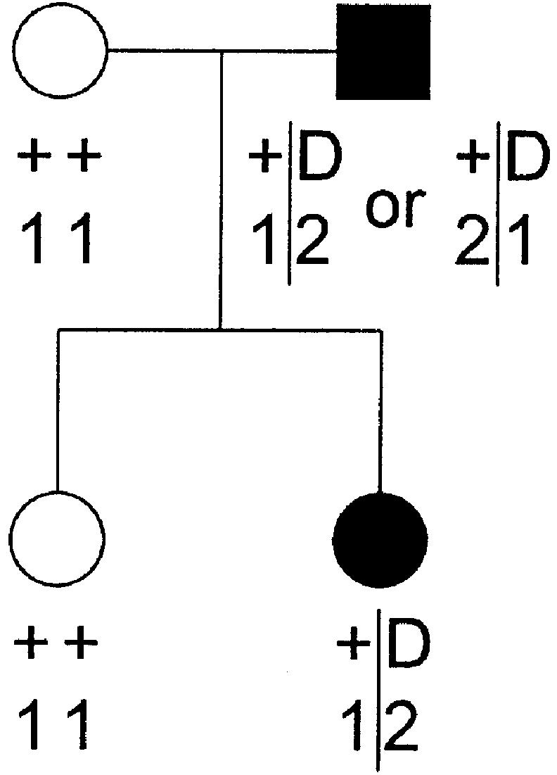
Example pedigree for likelihood computation that uses complex recombination fractions. The trait-locus genotypes are shown as inferred for a fully penetrant dominant disease. See text for the likelihood computation on this pedigree.
This example demonstrates that θ and ε are confounded in two-point analysis, but, as will be shown below, the two components become separable in multiple two-point and multipoint analysis.
The only effect of errors in inferred trait-locus genotypes discussed so far was misclassification of the genotype of children of parents with inferred genotype D/+ at the diallelic trait locus, since we implicitly focused only on truly informative meioses. In reality, however, not all meioses are informative for linkage, and errors in inferring trait-locus genotypes of a parent can make truly informative meioses (D/+) appear to be uninformative (D/D or ++) and vice versa. Figure 5 shows that our model also applies when one allows for misclassification of meiotic informativeness due to genotype errors. In that figure, the previously introduced misclassification probability, ε, of a true recombinant as a nonrecombinant, and vice versa, can be seen to be equal to 0.5ψ+ω(1-ψ) among meioses that are inferred to be informative (ψ is the proportion of truly uninformative meioses mistakenly assumed to be informative, and ω is the proportion of meioses from truly informative parents with misclassified recombination status). Meioses assumed to be uninformative are, naturally, not scored. This censoring of truly informative meioses does not lead to a bias in the recombination fraction but results in loss of information.
Figure 5.

Misclassification of recombination status in the presence of errors in assumed meiotic informativeness. This figure shows the relationship of the error component, ε, to misclassification of the recombination status and of meiotic informativeness. Note that the meiotic informativeness refers to the parental trait-locus genotype, whereas the observed recombination status refers to an offspring, in whom trait-locus genotype errors may also have occurred. The presented error model is still valid, with ε=0.5ψ+ω(1-ψ).
An implicit assumption made above is that the misclassification errors are independent for all meioses in a study. If the trait-locus genotype of a parent is incorrectly inferred, however, the recombination status of all of his children could be affected at the same time. In the case of a diallelic disease locus, however, every genotype error in a parent will lead to a change in meiotic informativeness of that parent. Since meioses that are assumed to be uninformative (assumed parental genotype D/D or +/+) are not analyzed, they contribute no false inference of meiotic recombination status at all. However, an uninformative parent whose genotype is incorrectly inferred to be D/+ will lead to 50% of his children having their recombination status misclassified (ε=0.5), although whether or not misclassification occurs is independent for each offspring. In reality, a fraction of all meioses will have one true value of ε, whereas, for the remaining meioses, the misclassification probability will be ε=0.5. Such “heterogeneity” of the misclassification rate could be dealt with by use of methods analogous to the way that heterogeneity of the recombination fraction is allowed for in linkage analysis (Smith 1963; Terwilliger 2000_a_). The effect of assuming “homogeneity” of the misclassification parameter for all meioses will be similar to the effect in sib-pair analysis of the use of the “mean test” (see Knapp et al. 1994) rather than the “possible triangle test” (see Holmans 1993), for which the assumption of independence of the meioses derived from the two parents (which underlies the mean test) give locally optimal performance (Knapp et al. 1994).
Because recombination fractions themselves are not additive (even when constrained to the real line, i.e., ε=0), it is useful to transform these probability measures into additive map-distance measures. Under the assumption of the Haldane (1919) mapping function, x(θ)=-0.5_ln_(1-2θ), for simplicity, although any map function can, in principle, be used, the individual components of the complex recombination fraction can be converted into additive map-distance measures to give the complex-valued distance vector X(Θ)=x(θ)+x(ε)i, with the real-valued map-distance metric being  (the subscript “ds” denotes “distance summing,” to distinguish this measure from the “ts” metric defined above in the complex probability space). The addition of θ and ε is done under the assumption that misclassification is independent of actual recombination, since there is no biological reason to assume otherwise.
The “ds” metric ( ) defines a well-known metric space (Nahin 1998, p. 244) often referred to as a taxicab geometry (Krause 1975), in which the vector sum is the sum of the orthogonal vector lengths. For a simple explanation of this metric, look at figure 6. Assume that a taxicab can only travel horizontally or vertically on a regular grid of streets. The distance from point A to point B is then the sum of the horizontal and vertical distances for a total of 2+1=3 blocks in this example. In contrast, the distance in Euclidean space, which also allows diagonal movement (“as the crow flies”), is
  . In any metric space, a circle is defined as the set of all points equidistant from some fixed point (the center of the circle; C in fig. 6; see Buskes and van Rooij 1997). In taxicab geometry, a circle looks like a Euclidean square, as described by Krause (1975). By direct analogy, in our “ds” mode, for any given value of the total recombination probability between marker and disease loci,
  , the set of all points equidistant from the fixed location of a marker locus (a taxicab circle) would likewise look like a square on the complex map-distance space. However, adding the restriction that ε⩾0, with no directional orientation of θ relative to the other marker loci on the chromosome, a taxicab semicircle,
  , would result, which looks like a right isosceles triangle in Euclidean space (fig. 7).
Figure 6.

Taxicab geometry. In “taxicab geometry,” only horizontal and vertical movement on a grid is allowed, just like the movement of a taxicab on a regular grid of city streets. The taxicab distance between two points (A and B) is therefore the sum of the horizontal and vertical distances between them, in this case 2+1=3. In contrast, in Euclidean geometry, where diagonal movement (“as the crow flies”) is also allowed, the distance between these two points is  . A taxicab circle (with radius 2), consisting of points equidistant from its center (C), is also shown and looks like a square in Euclidean space.
Figure 7.

Complex map distance. Since recombination fractions are not additive, it is useful to convert them into additive measures of genetic map distance. Figure 7 is the analog in complex map-distance space of figure 3 in complex recombination fraction space. For a given value of the total recombination probability,  , under the assumption of ε⩾0 and no directional orientation of θ relative to other marker loci, two edges of a right isosceles triangle are defined by the set
  .
.
Multiple Two-Point Analysis with Complex-Valued Recombination Fractions
Figures 8A and 8_B_ show two-point analysis and multiple two-point analysis, respectively, in terms of taxicab circles centered around each marker locus. Notice that, in two-point analysis (fig. 8A), the error components [ε_Di_ or x(ε_Di_) in complex map-distance space] are unconstrained [ε_Di_⩾0, x(ε_Di_)⩾0] and are allowed to vary for different marker loci. However, they are not estimated as separate components but are absorbed by inflated recombination fraction/map-distance estimates ( ,
,  ). The true location of the disease locus is typically inside the taxicab circles, as shown, because of the common overestimation of the recombination fraction, and the taxicab circles of different marker loci therefore do not normally intersect in one position on the chromosome. In multiple two-point linkage analysis (Morton 1988; Morton and Andrews 1989; Shields et al. 1991), the recombination fraction,
  , is estimated between each of a set of marker loci and the trait locus jointly, subject to the constraints imposed by the marker-marker linkage relationships. In other words, if the disease were assumed to be at map position D in the figure, the value of the recombination fraction between D and each of the marker loci would be fully determined, and the two-point LOD scores would be computed under these restrictions—that is, the taxicab semicircles from the two-point analyses would be forced to intersect on the real line, since ε is fixed at 0 (fig. 8B). The probability model for multiple two-point analysis is given in fig. 9A.
Figure 8.

Two-point and multiple two-point linkage analysis. In two-point linkage analysis (A), errors in the recombination fractions between each marker locus (M1, M2, M3) and the disease (D) are implicitly allowed through inflation of the recombination fraction estimate, but this error component is not estimated separately. Since the recombination fractions are typically overestimated, the triangles (corresponding to a specific map-distance estimate from each marker locus) are shown to extend beyond the true position of the trait locus. Not all triangles intersect at the same position, because the estimate of ε is not constrained to be equal for the different marker loci. In multiple two-point analysis without an error component (B), all triangles are forced to intersect on the chromosome at the assumed position of the disease gene, because of linearity constraints. When the error component is incorporated into this type of analysis (C), the triangles are still forced to intersect at the position of the trait locus—not necessarily on the chromosome but rather at some distance, x(ε), above in the error dimension.
Figure 9.

Multiple two-point and multipoint linkage analysis with complex recombination fractions. In multiple two-point linkage analysis without an error component (A), the recombination fractions between each marker locus and the disease locus are constrained by the map. An error component, ε, can be incorporated into multiple two-point analysis, as shown in (B). The real recombination fractions are again constrained, and only the error component—equal for all marker loci—is estimated. The last two panels show multipoint analysis without (C) and with (D) the error component. (Note that θ23 is used in multipoint analysis instead of θD3 in multiple two-point analysis.) The information provided by all marker loci is collapsed into a fictitious, highly informative marker locus at the assumed position of the trait locus, and linkage analysis is then performed between this hypothetical marker locus and the assigned trait-locus genotypes. In conventional multipoint analysis (C), the recombination fraction between this fictitious marker locus and the trait locus is fixed at 0, which is no longer the case when an error component is incorporated into the model (D), as proposed.
Extension of multiple two-point analysis to allow for the “imaginary” component of the recombination fraction vector to be >0 would be straightforward. Since ε is independent of the marker loci and merely is a function of the errors in the assignment of disease-locus genotypes, the actual value of parameter ε (not its estimate) can be shown to be theoretically identical for all marker loci used in the analysis. Thus, one additional parameter would have to be estimated in this multiple two-point approach with complex-valued recombination fractions. The real components, θ_Di_, of the complex recombination fractions, Θ_Di_, would remain constrained according to the chromosomal linkage map, whereas the imaginary component, ε, would be allowed to be nonzero but be constrained to some constant value in the analysis (equal for all marker loci). Thus, the maximum-likelihood estimates of the recombination fraction between each marker locus and the trait locus would be constrained to be  , for each marker locus i. The corresponding taxicab circle representation is shown in figure 8C. The taxicab circles are now constrained only to intersect at some point in the complex map-distance space at or above the assumed disease locus. If the imaginary component were estimated to be ε=0.5, then all of the pairwise recombination fractions would be 0.5 as well, according to the “ts” metric defined above. The probability model for “complex” multiple two-point analysis is shown in figure 9B.
Multipoint Analysis in the Complex Plane
If one considers the three marker loci shown in figures 8 and 9 (locus order M1-D-M2-M3), then the recombination status of the interval between D and M2 would also provide information about the recombination status between the disease and M3. Multipoint linkage analysis (Lathrop et al. 1984; Lander and Green 1987) takes this into account by analyzing recombination among all marker loci jointly. The probability model of multipoint analysis without an error component is shown in figure 9C. The likelihood of a meiosis with, say, a recombination between M1 and D, a recombination between D and M2, and no recombination between M2 and M3 would be θ_D_1θ_D_2(1-θ23), under the assumption of absence of interference. Under the null hypothesis of no linkage, the likelihood would be 0.5(1-θ12)(1-θ23) (because the assumed locus order then is M1-M2-M3, with D on another chromosome), and the likelihood ratio reduces to

which is only a function of the recombination fractions with the marker loci adjacent to the disease locus. (It should be noted that when the flanking marker loci are uninformative, the other marker loci do provide information about linkage but only indirectly, through their relationship to both the uninformative marker loci and the disease locus.) Analogous results can be obtained for the other possible multilocus recombination events. For this example, as θ12→0 (and therefore also θ_D_1→0 and θ_D_2→0), this likelihood ratio would approach 0, and the corresponding LOD score would go to −∞, since the disease locus is observed to recombine with each of the flanking marker loci, which is not possible when the recombination fractions are 0 and misclassification is not allowed.
In extending multipoint analysis to complex-valued recombination fractions (the probability model is shown in fig. 9D), one must allow for the two possible explanations of the observed meiosis above. Either there were true recombinations between both M1 and D and between D and M2 and no misclassification error, or else there was no recombination in either of the two intervals but an error in the trait-locus genotype assignment led to both apparent recombination events. The likelihood would then be (1-ε)θ_D_1θ_D_2(1-θ23)+ε(1-θ_D_1)(1-θ_D_2)(1-θ23) under the hypothesis of linkage at a given map position between marker loci M1 and M2. Under the null hypothesis of no linkage, the likelihood would again be 0.5(1–θ12)(1–θ23), as above. The resulting likelihood ratio for this specific type of meiosis, after cancellation of the term (1–θ23), would be
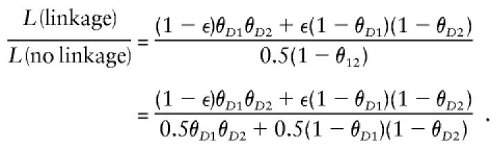
In this case, since the distance between the marker loci goes to 0, the likelihood ratio approaches ε/0.5, and the corresponding LOD score would thus be >-∞ as long as ε>0.
Notice that ε/0.5 is the same as the likelihood ratio (in one recombinant meiosis) in a two-point analysis with an informative marker locus positioned directly at the assumed genomic location of the disease gene, where  , as described above. A general proof of the equivalence of multipoint linkage analysis in the complex plane to traditional two-point linkage analysis is given in the Appendix. The only difference between “complex” multipoint analysis and two-point analysis is that data from multiple linked marker loci are jointly used to estimate the segregation pattern of chromosomal position x, rather than the single-marker locus at that position. The pointwise distribution of both LOD scores are identical. The genomewide behavior of this distribution has been described in detail (Dupuis et al. 1995; Lander and Kruglyak 1995; Terwilliger et al. 1997). By contrast, the conventional multipoint LOD score can be written in terms of ε as
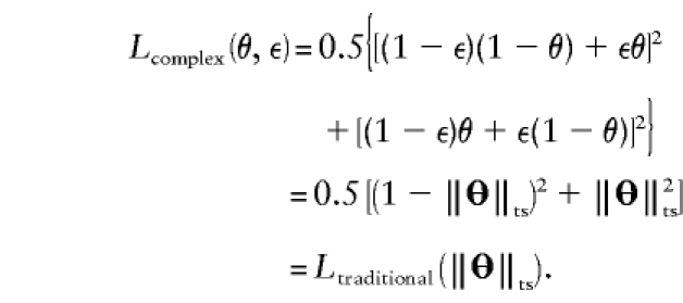
  for the same fixed map position x. Because of the lack of freedom in the alternative hypothesis, the hypotheses are not properly nested, and the distribution of the conventional multipoint LOD score, both pointwise and genomewide, is thus not well defined (see Terwilliger 2000_b_).
There is a penalty to be paid by “complex” multipoint analysis in comparison with conventional multipoint analysis, however, since the “complex” multipoint LOD score is always at least as large as its real-valued analog, owing to the existence of this extra parameter. A genome scan is not really a hypothesis-testing experiment, because nobody considers the null hypothesis to be that there is no gene. Rather, a genome scan is an estimation problem, where one attempts to localize the genomic position of the disease gene(s). The effect of allowing for nonzero values of ε in the analysis is to increase the size of the 3-LOD-unit support interval to which a disease gene might be localized. If the trait-locus genotypes were known without error, in M informative meioses, the expected width of the support interval would be 200/M cM, whereas, if one allows for trait-locus genotype errors by means of the misclassification parameter ε, the expected width of this support interval would be a function of the estimate of ε at the estimated map location of the disease gene. In figure 10, this relationship is graphed as the ratio of the mean width of the 3-LOD-unit support interval for given values of  to the expected width of the support interval for the traditional multipoint LOD score in the absence of trait-locus genotype-assignment errors (see Terwilliger 2000_b_ for further discussion of the genomewide properties of “complex” multipoint LOD scores). It should be noted that a single meiosis that is inferred falsely to be an obligate recombinant leads to an exclusion of the true location of the disease gene in conventional multipoint analysis, making the cost of adding this extra parameter minuscule compared with the cost of not allowing for it at all.
Figure 10.

Effect of the misclassification parameter ε on the expected 3-LOD-unit support interval for the disease locus. The effect of allowing for nonzero values of ε in the analysis is shown graphically, plotted as the ratio of the mean width of the 3-LOD-unit support interval (S.I.) for the disease locus for given values of  to the expected width of the interval for the traditional multipoint LOD score in the absence of trait-locus genotype assignment errors. Allowing for misclassifications greatly increases the width of the interval to which the disease gene can be localized. See Terwilliger 2000_b_ for more details.
Robustness of Multipoint Analysis with Complex Recombination Fractions
In traditional multipoint linkage analysis (without allowance for an imaginary error component in the recombination fraction), it is well known that errors in the genotype assignment at the disease-predisposing locus tend to push the disease “off the map” and lead to false exclusions of the true map position of the disease (see Risch and Giuffra 1992). This happens because, when the magnitude of the imaginary component of the recombination fraction is improperly assumed to be 0, all “imaginary recombination events” (due to improperly assigned trait-locus genotypes) appear as double recombinants on the real line of the chromosome. This in turn leads to false exclusions of linkage (negative LOD scores) at the true location of the disease locus. In comparison, two-point analysis is more robust to model errors (see Risch and Giuffra 1992). The reason is that false apparent recombinations can be absorbed in an inflated estimate of the recombination fraction, since the two components of the recombination fraction are completely confounded in two-point analysis. Because two-point analysis and multipoint analysis in the complex plane are equivalent, multipoint analysis, through the use of complex-valued recombination fractions, can be performed with the same degree of robustness to model errors at the trait locus as two-point analysis.
Discussion
In this article, an overview has been given of the role of mode-of-inheritance parameters in likelihood-based linkage analysis and of the effects of errors in these parameters on such methods. Since these parameters are never known with accuracy, particularly for complex traits—in which case they are not even particularly meaningful—it is important to develop methods that deal with the consequences of misspecifications in these parameters analytically. Here, recombination fractions defined in the complex number system, _C_1, are used to model the effects of errors in the assumed disease model, which can result in misclassification of the meiotic recombination status. Although marker-locus genotypes were implicitly assumed to be known with accuracy throughout this article, they are, of course, also subject to errors. Some of these errors can be treated in a similar manner, as described in the companion article (Göring and Terwilliger 2000_a_). Other types of errors associated with marker loci and their map can be accommodated through the use of profile likelihoods (Göring and Terwilliger 2000_b_), with or without conjunction to the complex-valued recombination fractions described in this article.
Risch and Giuffra (1992) originally proposed to circumvent the problems imposed by inaccuracies in the genotype assignment in “model-based” linkage analysis by specifying mode-of-inheritance models that led to less deterministic assignment of trait-locus genotypes on the basis of the observed phenotypes (i.e., “weak” models with low penetrance, high phenocopy rate, and/or high disease-allele frequency, leaving great ambiguity about the trait-locus genotypes). This approach does indeed diminish the risk of false-negative results in multipoint analysis but also leads to substantial loss of power (Clerget-Darpoux et al. 1986; Göring and Terwilliger 2000_c_). As the model becomes increasingly weaker, this ultimately results in the situation where the trait-locus genotypes of all pedigree members are completely unknown, in which case a pedigree provides no linkage information whatsoever. The reason why the risk of finding false-negative results is reduced by a “weak” model is that the prior probability of each admissible constellation of trait-locus genotypes would not differ that much, and, thus, when maximizing the overall likelihood over the recombination fraction, the posterior probability of each trait-locus genotype combination can be greatly affected by the observed marker-locus data. In contrast, when a strong genotype-phenotype relationship is assumed, the posterior probability of each trait-locus genotype constellation is dominated by the prior.
Throughout this article, we have described complex-valued recombination fractions in the context of “model-based” linkage analysis. However, the approach is also directly applicable to “model-free” methods, as shown elsewhere (Göring and Terwilliger 2000_c_). In fact, this proposal developed from an attempt to compare multipoint “model-based” and “model-free” methods, to understand why the latter is often claimed to be more robust than the former. The difference in robustness is due to the fact that “model-free” multipoint methods implicitly allow for an error component in the recombination fraction (e.g., Kruglyak and Lander 1995; Almasy and Blangero 1998), for the reason that the estimated parameter is typically not expressed as a recombination fraction (Göring and Terwilliger 2000_c_; Terwilliger and Göring 2000). Complex-valued recombination fractions are thus not only a means by which “model-based” multipoint analysis can be performed in a way that has the same robustness to model errors as two-point analysis, as shown in this article, but, in addition, the equivalence of most of the popular “model-free” analysis methods to certain forms of “model-based” analysis can be extended from the two-point case to the multipoint situation through the use of complex-valued recombination fractions (see Knapp et al. 1994; Trembath et al 1997; Göring and Terwilliger 2000_c_).
Acknowledgments
A Hitchings-Elion Fellowship from the Burroughs-Wellcome Fund (to J.D.T.) is gratefully acknowledged, as is grant HG00008 from the National Institute of Health to Jürg Ott (thesis advisor of H.H.H.G.).
Appendix: Proof of Equivalence of “Complex” Multipoint LOD-Score Analysis and Traditional Two-Point LOD-Score Analysis
Theorem: The “complex” multipoint LOD score is equivalent to the conventional two-point LOD score.
Proof: Let us assume that we want to test whether the disease locus (D) is at position x in the genome, flanked by two marker loci (M1 and M2) at recombination fractions θ_x_1 and θ_x_2, respectively. The distance between marker loci M1 and M2 is θ12=θ_x_1+θ_x_2-2θ_x_1θ_x_2, under the assumption of absence of interference (Haldane 1919). Under the null hypothesis, the disease locus is unlinked to the marker-locus map (θ_D_1=0.5), whereas, under the alternative hypothesis, the disease locus is at position x. The only way to observe recombination would be if disease-locus genotypes were misclassified, and thus P(recombination between x and D)=ε. The eight possible meiotic types are shown in table 1. In table 1 (top), the probability of each outcome is given under the hypothesis that the disease locus is at position x, and in table 1 (bottom) the probability of each outcome is given under the hypothesis that the disease locus is unlinked to the marker-locus map (θ_D_1=0.5).
Table 1.
List of all possible meiotic types, and their probabilities, for analysis of a disease locus (D) and two linked marker loci (M1, M2), for the alternative hypothesis of linkage (top) and the null hypothesis of no linkage (bottom).
| Recombination Status in Interval (locus orderM1-(x, D)-M2) | ||||
|---|---|---|---|---|
| Meiotic Type | M1-x | _x_-M2 | _x_-D | Probability |
| Y1 | N | N | N | (1-ε)[1-θ_x_1)(1-θ_x_2)] |
| Y2 | N | R | N | (1-ε)[(1-θ_x_1)θ_x_2] |
| Y3 | R | N | N | (1-ε)[θ_x_1(1-θ_x_2)] |
| Y4 | R | R | N | (1-ε)[θ_x_1θ_x_2] |
| Y5 | N | N | R | ε[(1-θ_x_1)(1-θ_x_2)] |
| Y6 | N | R | R | ε[(1-θ_x_1)θ_x_2] |
| Y7 | R | N | R | ε[θ_x_1(1-θ_x_2)] |
| Y8 | R | R | R | ε[θ_x_1θ_x_2] |
| Recombination Status in Interval (locus order D…M1-(x)-M2; θ_D_1=0.5) | ||||
| D–M1 | M1–x | _x_–M2 | ||
| Y1 | N | N | N | 0.5[(1-θ_x_1)(1-θ_x_2)] |
| Y2 | N | N | R | 0.5[(1-θ_x_1)θ_x_2] |
| Y3 | R | R | N | 0.5[θ_x_1(1-θ_x_2)] |
| Y4 | R | R | R | 0.5[θ_x_1θ_x_2] |
| Y5 | R | N | N | 0.5[(1-θ_x_1)(1-θ_x_2)] |
| Y6 | R | N | R | 0.5[(1-θ_x_1)θ_x_2] |
| Y7 | N | R | N | 0.5[θ_x_1(1-θ_x_2)] |
| Y8 | N | R | R | 0.5[θ_x_1θ_x_2] |
Proposition 1: The “complex” multipoint LOD score is equivalent to the “complex” two-point LOD score.
Proof: The “complex” multipoint LOD score can be written as follows:
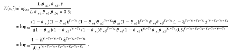
If “complex” two-point linkage analysis were done with a single-marker locus directly at position x, the meiosis types shown in table 1 (top) would be completely described by using only the last column, the recombination status between position x and the disease locus. In “complex” two point analysis, the frequency of an observed recombination between a marker locus (at position x) and the trait locus would be  . Writing out the “complex” two-point LOD score, we obtain
Because one cannot separate the components θ and ε in  , we can arbitrarily set θ=0 and thus eliminate one parameter from the equation, as follows:

This is exactly the same formula as for the “complex” multipoint LOD score.
Proposition 2: The “complex” two-point LOD score is equivalent to the conventional two-point LOD score.
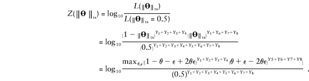
Proof: The “complex” two-point LOD score, however, can also be formulated under the condition where, rather than arbitrarily setting θ=0 and letting ε vary, ε=0 and θ is allowed to vary, as follows:

This formula, however, is exactly the same as for the conventional two-point LOD score between a marker locus at position x and a disease locus, with no allowance for misclassification.
By proposition 1, the “complex” multipoint LOD score was shown to be equivalent to the “complex” two-point LOD score, and by proposition 2, the “complex” two-point LOD score was shown to be equivalent to the conventional two-point LOD score. It follows directly that the “complex” multipoint LOD score is equivalent to the conventional two-point LOD score. The only difference is that the multipoint LOD score may be able to use more information—by using additional marker loci to determine the inheritance of position _x_—to determine the recombination status between position x and the inferred disease-locus genotypes.
References
- Almasy L, Blangero J (1998) Multipoint quantitative linkage analysis in general pedigrees. Am J Hum Genet 62:1198–1211 [DOI] [PMC free article] [PubMed]
- Buskes G, van Rooij A (1997) Topological spaces—from distance to neighborhood. Springer Verlag, New York [Google Scholar]
- Clerget-Darpoux F, Bonaïti-Peilié C, Hochez J (1986) Effects of misspecifying genetic parameters in LOD score analysis. Biometrics 42:393–399 [PubMed]
- Dupuis J, Brown PO, Siegmund D (1995) Statistical methods for linkage analysis of complex traits from high-resolution maps of identity by descent. Genetics 140:843–856 [DOI] [PMC free article] [PubMed]
- Göring HHH, Terwilliger JDT (2000_a_) Linkage analysis in the presence of errors II: marker-locus genotyping errors modeled with hypercomplex recombination fractions. Am J Hum Genet 66:1107–1118 (in this issue) [DOI] [PMC free article] [PubMed] [Google Scholar]
- ——— (2000_b_) Linkage analysis in the presence of errors III: marker loci and their map as nuisance parameters. Am J Hum Genet (in press) [DOI] [PMC free article] [PubMed] [Google Scholar]
- ——— (2000_c_) Linkage analysis in the presence of errors IV: joint pseudomarker analysis of linkage and/or linkage disequilibrium on a mixture of pedigrees and singletons when the mode of inheritance cannot be accurately specified. Am J Hum Genet (in press) [DOI] [PMC free article] [PubMed] [Google Scholar]
- Haldane JBS (1919) The combination of linkage values and the calculation of distances between the loci of linked factors. J Genet 8:299–309 [Google Scholar]
- Holmans P (1993) Asymptotic properties of affected-sib-pair linkage analysis. Am J Hum Genet 52:362–374 [PMC free article] [PubMed]
- Jaynes ET (1996) Probability theory: the logic of science. http://bayes.wustl.edu/etj/prob.html
- Keats BJB, Sherman SL, Morton NE, Robson EB, Buetow KH, Cann HM, Cartwright, PE et al (1991) Guidelines for human linkage maps: an international system for human linkage maps (ISLM, 1990). Genomics 9:557–560 [DOI] [PubMed]
- Knapp M, SA Seuchter, MP Baur (1994) Linkage analysis in nuclear families: relationship between affected sib-pair tests and LOD score analysis. Hum Hered 44:44–51 [DOI] [PubMed]
- Krause EF (1975) Taxicab geometry—an adventure in non-Euclidean geometry. Addison-Wesley, Menlo Park [Google Scholar]
- Kruglyak L, Lander ES (1995) Complete multipoint sib-pair analysis of qualitative and quantitative traits. Am J Hum Genet 57:439–454 [PMC free article] [PubMed]
- Lander ES, Green P (1987) Construction of multilocus genetic linkage maps in humans. Proc Natl Acad Sci USA 84:2363–2367 [DOI] [PMC free article] [PubMed]
- Lander ES, Kruglyak L (1995) Genetic dissection of complex traits: guidelines for interpreting and reporting linkage results. Nat Genet 11:241–247 [DOI] [PubMed]
- Lathrop, GM, Lalouel JM, Julier C, Ott J (1984) Strategies for multilocus linkage analysis in humans. Proc Natl Acad Sci USA 81:3443–3446 [DOI] [PMC free article] [PubMed]
- Martinez M, Khlat M, Leboyer M, Clerget-Darpoux F (1989) Performance of linkage analysis under misclassification error when the genetic model is unknown. Genet Epidemiol 6:253–258 [DOI] [PubMed]
- Morton NE (1955) Sequential tests for the detection of linkage. Am J Hum Genet 7:277–318 [PMC free article] [PubMed] [Google Scholar]
- ——— (1988) Multipoint mapping and the emporer's clothes. Ann Hum Genet 52:309–318 [DOI] [PubMed]
- Morton NE, Andrews V (1989) MAP, an expert system for multiple pairwise linkage analysis. Ann Hum Genet 53:263–269 [DOI] [PubMed]
- Nahin PJ (1998) An imaginary tale—the story of
 . Princeton University Press, Princeton, NJ [Google Scholar]
 - Ott J (1977) Linkage analysis with misclassification at one locus. Clin Genet 12:119–124 [erratum in (1977) Clin Genet 12:254] [DOI] [PubMed]
- ——— (1985) Analysis of human genetic linkage, 1st ed. Johns Hopkins University Press, Baltimore, MD [Google Scholar]
- Risch N, Giuffra L (1992) Model misspecification and multipoint linkage analysis. Hum Hered 42:77–92 [DOI] [PubMed]
- Sarkar S (1998) Genetics and reductionism. Cambridge University Press, Cambridge, UK [Google Scholar]
- Shields DC, Collins A, Buetow KH, Morton NE (1991) Error filtration, interference, and the human linkage map. Proc Natl Acad Sci USA 88:6501–6505 [DOI] [PMC free article] [PubMed]
- Smith CAB (1963) Testing for heterogeneity of recombination fraction values in human genetics. Ann Hum Genet 27:175–182 [DOI] [PubMed] [Google Scholar]
- Smith HF (1937) Test of significance for Mendelian ratios when classification is uncertain. Ann Eugen 8:94–95 [Google Scholar]
- Terwilliger JD (1998) Linkage analysis, model-based. In: Armitage P, Colton T (eds) Encylopedia of biostatistics. John Wiley and Sons, Chichester, UK, pp 2279–2291 [Google Scholar]
- ——— (2000_a_) A likelihood-based extended admixture model of oligogenic inheritance in “model-based” or “model-free,” two-point or multi-point, linkage and/or LD analysis. Eur J Hum Genet (in press) [DOI] [PubMed] [Google Scholar]
- ——— (2000_b_) On the resolution and feasibility of genome scanning approaches to unraveling the genetic components of multifactorial phenotypes. In: Rao DC, Province MA (eds) Genetic dissection of complex phenotypes: challenges for the new millennium. Academic Press, San Diego (in press) [Google Scholar]
- Terwilliger JD, Göring HHH (2000) A review of gene mapping in the 20th and 21st centuries: statistical methods, data analysis, and experimental design. Hum Biol 72:63–132 [PubMed] [Google Scholar]
- Terwilliger JD, Ott J (1994) Handbook of Human Genetic Linkage. Johns Hopkins University Press, Baltimore, MD [Google Scholar]
- Terwilliger JD, Shannon WD, Lathrop GM, Nolan JP, Goldin LR, Chase GA, Weeks DE (1997) True and false positive peaks in genomewide scans: applications of length-biased sampling to linkage mapping. Am J Hum Genet 61:430–438 [DOI] [PMC free article] [PubMed]
- Trembath RC, Clough RL, Rosbotham JL, Jones AB, Camp RDR, Frodsham A, Browne J, et al (1997) Identification of a major susceptibility locus on chromosome 6p and evidence for further disease loci revealed by a two stage genome-wide search in psoriasis. Hum Molec Genet 6:813–820 [DOI] [PubMed]
- Walley P (1991) Statistical reasoning with imprecise probabilities. Chapman and Hall, London [Google Scholar]