Elasticity of Short DNA Molecules: Theory and Experiment for Contour Lengths of 0.6–7 μm (original) (raw)
Abstract
The wormlike chain (WLC) model currently provides the best description of double-stranded DNA elasticity for micron-sized molecules. This theory requires two intrinsic material parameters—the contour length L and the persistence length p. We measured and then analyzed the elasticity of double-stranded DNA as a function of L (632 nm–7.03 _μ_m) using the classic solution to the WLC model. When the elasticity data were analyzed using this solution, the resulting fitted value for the persistence length _p_wlc depended on L; even for moderately long DNA molecules (L = 1300 nm), this apparent persistence length was 10% smaller than its limiting value for long DNA. Because p is a material parameter, and cannot depend on length, we sought a new solution to the WLC model, which we call the “finite wormlike chain (FWLC),” to account for effects not considered in the classic solution. Specifically we accounted for the finite chain length, the chain-end boundary conditions, and the bead rotational fluctuations inherent in optical trapping assays where beads are used to apply the force. After incorporating these corrections, we used our FWLC solution to generate force-extension curves, and then fit those curves with the classic WLC solution, as done in the standard experimental analysis. These results qualitatively reproduced the apparent dependence of _p_wlc on L seen in experimental data when analyzed with the classic WLC solution. Directly fitting experimental data to the FWLC solution reduces the apparent dependence of _p_fwlc on L by a factor of 3. Thus, the FWLC solution provides a significantly improved theoretical framework in which to analyze single-molecule experiments over a broad range of experimentally accessible DNA lengths, including both short (a few hundred nanometers in contour length) and very long (microns in contour length) molecules.
INTRODUCTION
Protein-nucleic acid interactions are essential to life and govern fundamental genomic processes such as replication, transcription, translation, splicing, and DNA repair. Early single-molecule experiments yielded new insight into the mechanical behavior of individual DNA molecules (1–4). Subsequently, single-molecule force experiments investigated diverse proteins that interact with DNA, including polymerases (5–10), helicases (11–16), phage portal proteins (17), topoisomerases (18), exonucleases (19,20), endonucleases (21), and histones (22,23). In one realization of common experimental geometries (Fig. 1), a processive nucleic-acid enzyme, bound to a DNA molecule, is anchored to a surface (24). The other end of the DNA molecule is attached to a bead held in an optical trap. The introduction of ATP (or NTPs) leads to enzymatic motion that shortens the DNA molecule and pulls on the trapped bead. These experiments lead to important kinetic parameters of individual enzymes, such as translocation rate (5–10,12–17), pause frequency and duration (6,19), and step size (13,25). Moreover, the application of force allows the enzyme's motion to be measured as a function of applied load (5,7,8,17,21).
FIGURE 1.

Cartoon illustrating the experimental geometry (not to scale). A DNA molecule (green) is linked at one end to a surface. The opposite end of the DNA is attached to a bead held in an optical trap (orange). The trap center is offset a lateral distance _x_DNA from the surface attachment point. The vertical distance of the trap center from the surface is _z_trap. The bead displacement in both axes (_x_bd and _z_bd) is measured from the center of the trap (dashed line) to the center of the bead (solid line). The extension, x, of the DNA along the stretching axis can be determined from the geometry (24).
Single-molecule force experiments, independent of the specific experimental geometry, require a model to deduce the polymer's intrinsic contour length (L) from measurements of force and extension (24). This force-independent length allows accurate comparison between ensemble biochemical translocation rates (measured in basepairs/s) and physical velocities (nm/s) measured in single-molecule assays.
To date, the wormlike chain model (WLC) provides the best description of double-stranded DNA elasticity (4,24,26,27) for micron-sized molecules and is the definitive model for interpreting single-molecule protein-DNA experiments. Moreover, the WLC has become the standard model for characterizing the elastic properties of RNA (28) and proteins (29). The WLC predicts the average end-to-end extension x of a semiflexible polymer given a force F applied to the ends of the molecule. The theory requires two intrinsic material parameters, i.e., the contour length L and the persistence length p. The contour length is equal to the number of monomers in the chain times the distance per monomer (0.338 nm/bp for B-form DNA). The persistence length characterizes the bending stiffness of the polymer and depends on the molecule's local elastic behavior. While there is a slight ionic dependence, for dsDNA p ≈ 50 nm, as determined by traditional bulk techniques (30,31) and more recently by single-molecule experiments (2,4,24,26).
The standard mathematical treatment of the WLC, which relates F to the fractional extension x/L (26), is exact in the limit L/p → ∞. Yet single-molecule experiments with dsDNA molecules (and other double-stranded nucleic acids) often use short (32) to moderate length (9) molecules where L/p ∼ 6–20. Failure of the WLC solution to accurately describe DNA elasticity over this range of lengths could lead to incorrect determination of p, L, and hence enzymatic rates. Precise knowledge of L allows enzymatic pauses to be related to the underlying DNA sequence (19,33). Accurate measurement of p verifies that only a single molecule of DNA links a bead to a surface (24). Therefore, correct modeling of DNA elasticity over a range of lengths is essential to the precise and accurate analysis of single molecule experiments.
To investigate the potential limitations of the WLC solution, we performed a combined experimental and theoretical study of DNA elasticity for commonly used contour lengths. First, we measured and then analyzed the elasticity of dsDNA as a function of L using the classic WLC solution. The successful theory, applied to experimental data, should yield a fitted value of p independent of L, since p is a local, intrinsic property of the polymer. However, when the elasticity data were analyzed using the classic WLC solution, the inferred value of p, which we will call _p_wlc, depended on L for contour lengths over the range 632 nm to 7.030 _μ_m. We reasoned that such an unphysical length dependence of the apparent persistence length may occur because the traditional WLC solution does not include finite-length effects.
Thus, we developed the finite wormlike chain (FWLC) solution by including three effects important to experiments: the finite length of the chain, rotational fluctuations of the bead, and the boundary conditions at the chain's anchor points. We incorporated finite-length effects and the boundary conditions by using a mathematical formulation of the WLC which is accurate for arbitrary L/p and specifying the boundary conditions at each end of the polymer. We addressed bead rotations by averaging over rotational fluctuations. Typically, experiments measure the bead's position; molecular extension is then calculated by subtracting the bead's radius. This analysis is only correct when the polymer-bead attachment is in line with the direction of the force. For typical experiments where the bead is not rotationally constrained, bead rotational fluctuations introduce an error in this measurement. For polymers with L <1.3 _μ_m (_L_/_p_ ≤ 25), we show that these effects are significant (>10%). This work is related to previous theoretical results on the stretching of extremely short polymers (L ∼ p), including exact analytic results in the rodlike limit (34) and Monte Carlo simulations for rodlike polymers under tension (35). Our article gives analytic approximations for any length polymer and includes bead rotational fluctuations that we show are important for analyzing experiments.
To demonstrate the validity of the FWLC, we predicted force-extension curves with the FWLC and fit using the classic WLC solution. These results qualitatively captured the apparent reduction of p with L seen in experimental data fit with the classic WLC solution. Additionally, directly fitting experimental data to the FWLC solution reduces the dependence of p on L by a factor of three. Thus, the FWLC solution provides a significantly improved theoretical framework in which to analyze single-molecule experiments over a broad range of experimentally accessible DNA lengths, from hundreds of nanometers to microns.
MATERIALS AND METHODS
DNA ladder synthesis and sample preparation
We prepared double-stranded DNA by polymerase chain reaction (PCR; GeneAmp XL PCR Kit, Applied Biosystems, Foster City, CA) using one digoxigenin-labeled and one biotin-labeled primer (Integrated DNA Technologies, Coralville, IA). These labels enabled us to attach a DNA molecule at one end to a streptavidin-coated coverslip and at the other end to an anti-digoxigenin coated bead. DNA molecules ranging in size from 1870 to 7138 bp were amplified using double-stranded M13 Phage DNA (M13mp18 plasmid, Bayou Biolabs, Harahan, LA) as the template. For the longest DNA studied (20.8 kbp), we used a portion of the _λ_-bacteriophage genome supplied with the XL PCR kit. The PCR products were purified from agarose gels (QIAquick Gel Extraction Kit, QIAGEN, Valencia, CA). We prepared anti-digoxigenin beads by covalently attaching anti-digoxigenin to aldehyde-sulfate beads (0.49 _μ_m; Interfacial Dynamics, Portland, OR), following the protocol adapted from Interfacial Dynamics. We prepared bead-DNA complexes by mixing beads and DNA (5:1 ratio; ∼250 pM beads) in wash buffer (WB; 20 mM Tris-HCl, pH 7.5, 100 mM KCl, and 3 mg/ml bovine serum albumin, i.e., BSA) for 30 min. Before use, buffers were filtered through 0.2 _μ_m filters. Experiments were done in epoxy-stabilized flow cells (19) with a sample volume of 15 _μ_l constructed with KOH-cleaned microscope coverslips, double sticky tape, five-minute epoxy, and microscope slides. We initially incubated the flow cells with biotinylated BSA (125 _μ_g/ml in 100 mM phosphate buffer, pH 7.5; Vector Laboratories, Burlingame, CA) for 30 min. After washing with WB, we incubated the flow cells with streptavidin (10 _μ_g/ml in WB; Vector Laboratories) for 15–20 min. After further washing, we flowed bead-DNA complexes into the flow cells at 370 pM beads. After 20 min, we washed the flow cells with 1 ml of stretching buffer (10 mM phosphate buffer, pH 7.5; and 3 mg/ml BSA, TWEEN-20) and sealed them with nail polish. This ionic condition was chosen to match previous measurements reported by Wang et al. (24).
Optical trap
Our optical trapping microscope, based on earlier work (36,37), used a 1064-nm laser for trapping and an 810-nm laser for deducing bead motion via back-focal plane detection (38). From the light incident on the quadrant photodiode, we determined the normalized difference along the x and y axes using custom-built electronics (bandwidth, as tested by a blinking 850-nm diode, is ∼250 kHz) with built-in programmable anti-aliasing filters. The normalized differences of the quadrant photodiode electronics, as well as the sum signal, were digitized at 16-bit resolution. To convert volts to position, we first needed to calibrate a closed-loop PZT mirror (S-330.2SL, Physik Instrumente, Karlsruhe, Germany). This PZT mirror was imaged by a pair of lenses onto the back focal plane of the microscope objective such that rotations of the mirror led to translations of the laser focus in the microscope's imaging plane. We calibrated the PZT mirror by scanning a stuck bead in a grid using a calibrated three-axis closed-loop PZT stage (P517.3CD, Physik Instrumente) and determining the PZT mirror voltages associated with the center of the stuck bead at each stage position. After this one time-calibration, we could translate an optically trapped bead through the fixed, stationary detector beam to generate a Volts-per-nanometer reference curve.
Trap stiffness, at six different laser powers, was determined using the equipartition theorem at a trap height of 445 nm from the surface and verified to within 3% using power spectral analysis. As expected, this calibration yielded a linear relationship between trap stiffness and optical power that was used in subsequent DNA stretching experiments.
DNA stretching and data analysis
To compute the DNA's elasticity accurately, the location of the DNA's attachment to the cover glass, i.e., its tether point, must be accurately aligned to the optical trap. The tether point's vertical position was found by monitoring the change in forward-scattered light as a trapped, tethered bead was brought into surface contact by raising the stage (19). The PZT stage was then lowered by 300 nm, though the trap's motion is attenuated ≈20% because of the index of refraction difference between the cover glass and the water (39). We next performed a two-dimensional elasticity-centering procedure using the instrument in a position-clamp mode (24). To minimize vertical motion of the bead in the optical trap, we set the position clamp to 40 nm from the trap center. For the shortest molecules studied, this corresponds to (at most) an 80-nm displacement in z. Nonetheless, we made sure that the sensitivity in x changed <1% over 200-nm vertical displacement of a bead relative to the trap center. With an initial trap stiffness of 0.03 pN/nm, the position clamp became active at 1.2 pN. After two rounds of this _x_-y alignment and a second round of vertical alignment, we measured the elasticity of the DNA along the x axis in response to stretching in both the positive and negative directions. At each extension, we digitized 2000 or 5000 data points at 120 kHz, depending on the applied force. We increased the extension by moving the PZT stage in increments of 1–10 nm depending on the length of the DNA substrate and the applied force. The resulting one-dimensional elasticity curve was analyzed based on the two-dimensional experimental geometry (24) to generate the extension and force along the stretching axis. We fit each F versus x trace to an improved analytic approximation of the WLC solution (26), which was symmetrized to simultaneously fit the data for both positive and negative stretching relative to the tether point. This fit returns three values, _p_wlc, L, and Δ, where _p_wlc is the apparent persistence length, L is the contour length, and Δ is the location of the tether point.
THEORY
WLC solution
Here we review the basic assumptions of the WLC solution, then describe extensions to the usual WLC solution necessary to describe the elastic properties of relatively short molecules in different experimental geometries (Fig. 2).
FIGURE 2.

Sketch of idealized experimental geometries for single-molecule force experiments with nucleic-acid polymers. The total molecule extension is x. (A) Idealized pulling geometry in which force is applied directly to the ends of the molecule. (B) One-bead geometry. The molecule is attached at one end to a surface (glass slide or coverslip) and at the other end to a bead. Force is applied to the center of the bead. (C) Two-bead geometry. The molecule is attached at both ends to beads.
The WLC model assumes an inextensible polymer: the contour length L of the molecule cannot be changed by applied force. For double-stranded DNA, the overstretching transition, which occurs for an applied force ∼60 pN, is a dramatic change in contour length; however, lower applied forces (up to ∼10 pN) respect the inextensibility constraint (26,40,41). The polymer is assumed to possess an isotropic bending rigidity, characterized by the persistence length, p. The persistence length is the length scale over which thermal fluctuations randomize the chain orientation. In principle, the rod also resists twist. However, in many experiments, including ours, the twist is unconstrained and can be ignored. We note that when considering single finite-length molecules, we are not working in any “thermodynamic limit.” Therefore, different ensembles are not equivalent (42–44). At very low forces, which we will not consider here, another effect complicates the relation between ensembles (see (57)). In this article, we work in the ensemble relevant to most experiments where the applied force is fixed, and we calculate the extension.
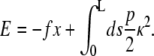
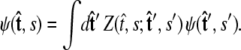
The WLC is formulated in terms of the WLC energy, which includes the bending energy (Hooke's law in the chain curvature) and the work done by the applied force. The WLC energy (in units of the thermal energy k_B_T) is
 |
(1) |
|---|
Here f (F divided by the thermal energy k_B_T) is applied in the  direction, s denotes arc length, and the total extension of the chain is x. The curvature can be defined in terms of arc-length derivatives of the chain coordinate (Fig. 3). If the chain conformation is described by a space curve r(s) and the unit vector tangent to the chain is
  then
then 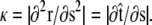 Note that the chain extension can be calculated as
FIGURE 3.

Variables used to describe chain conformations. Force is applied in the  direction. The arc length along the chain is s, and the vector r(s) = (x(s), y(s), z(s)) is the coordinate of the chain at arc length s. The vector
  is the unit vector tangent to the chain at s.
We assume that the force is applied in the  direction, as sketched in Fig. 2. In the experiments, the force is typically applied not directly in the
  direction, but at an angle to the surface (Fig. 1).
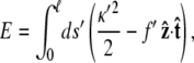
We rescale by dividing all lengths by the persistence length p, so the scaled energy is
 |
(2) |
|---|
where ℓ = L/p, f ′ = fp, _s_′ = s/p, and _κ_′ = κp. We will drop the primes in the remainder of the article.
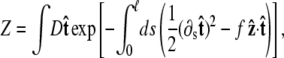
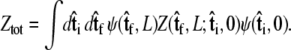
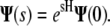
To determine the extension for a given applied force requires averaging over different polymer conformations. This leads to a path integral formulation of the statistical-mechanics problem in the tangent vector to the chain (31,45). If the ends of the chain are held at fixed orientations, the partition function of the chain is
 |
(3) |
|---|
where the integral in  is over all possible paths between the two endpoints of the chain with the specified orientations. The partition function can be reformulated as a propagator. (We use notation where the total probability amplitude is denoted by Z or _Z_tot, and the propagator, a conditional probability distribution, is denoted by
  Both of these quantities are referred to as the partition function in the literature.) The propagator connects the probability distribution for the tangent vector at point s,
  to the same probability distribution at point _s_′:
 |
(4) |
|---|
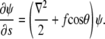
From this relation, one can derive a Schrödinger-like equation which describes the s evolution of ψ (4):
 |
(5) |
|---|
Here ∇2 is the two-dimensional Laplacian on the surface of the unit sphere, and 
Boundary conditions at chain ends
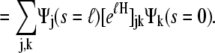
For relatively short polymers, the boundary conditions at the ends of the chain must be considered (46). The boundary conditions are specified by two probability density functions,  and
and  Our goal is to use these two constraints and the propagator
  to determine the total partition function _Z_tot. Physically, this corresponds to beginning with
  the initial probability distribution for the tangent angle at the s = 0 end of the chain, and then applying the propagator
  to determine the probability distribution at the other end of the chain. However, the calculated distribution at the end of the chain,
  does not necessarily correspond to the specified boundary condition
  To integrate the constraint on the tangent vector at s = L with the Markovian relation given by Eq. 4, we project the s = L probability distribution onto the boundary condition, or, alternatively, imagine propagating to s = L – ε and then demanding that ψ be continuous via a Dirac δ function,
  In this case, we find
 |
(6) |
|---|
If we perform the integration over  then we can write the projection as
 |
(7) |
|---|
In this article, we will focus on three specific boundary conditions: unconstrained, half-constrained, and normal, which are sketched in Fig. 4, A_–_C, and described in more detail below.
FIGURE 4.

Sketch of the boundary conditions. (A) Unconstrained boundary conditions. The tangent vector at the end of the chain (short arrow) points in any direction relative to the direction of applied force (notched arrowhead). (B) Half-constrained boundary conditions. Due to a constraint (such as the presence of a solid surface), the tangent vector at the end of the chain can point only in the upper half-sphere. (C) Perpendicular boundary conditions. The tangent vector is constrained to point only normal to the surface in the direction of the applied force. (Note that boundary conditions are necessary for both ends (s = 0 and s = L) of the chain.) (D) Variables used to describe bead rotational fluctuations. The vector  points from the center of the bead to the polymer-bead attachment. The angle θ between the
  direction and the bead-chain attachment is defined by
  The angle γ is defined by
  where
where  is the tangent vector at the end of the chain. The bead has radius R.
Bead rotational fluctuations
Force in single-molecule experiments is typically applied through a bead, which rotates due to thermal fluctuations. The rotational fluctuations of the bead can be explicitly included in the theory. Here we consider the experimental configuration with a bead at one end of the chain with the other end of the chain fixed to a surface (the geometry is sketched in Fig. 2 B; generalization to an experimental configuration with a bead at each end of the polymer is straightforward). In this case, the theory predicts the extension to the center of the bead as measured in the experiments, not just the molecule extension. We assume that the bead is spherical and the fluctuations in the polymer-bead attachment are azimuthally symmetric about the  axis.
axis.
The unit vector  points from the center of the bead to the polymer-bead attachment, as sketched in Fig. 4 D. Thus the bead's contribution to the energy of a fluctuation with a given
  is
is  where R is the bead radius. Note that the energy is minimized when
  and for other bead orientations, the energy increases. This gives a restoring torque on the bead that increases as FR increases. We write the rescaled energy including this term as
 |
(8) |
|---|
where r = R/p. The partition function of the chain is
 |
(9) |
|---|
where the first integral is over all possible paths between the two endpoints of the chain, and the second integral is over all allowable vectors  Below we evaluate the second integral, thereby performing the average over fluctuations in
MATHEMATICAL METHODS
To calculate of the force-extension relation, the main quantity of interest in single-molecule experiments, we must first calculate the tangent-vector probability distribution  for all s along the chain. The distribution satisfies Eq. 5 above. This partial differential equation can be solved using separation of variables in s and
  where the angular dependence is expanded in spherical harmonics (4).
 |
(10) |
|---|
Each value of j corresponds to a different component of Ψ. We assume azimuthal symmetry, so only the m = 0 spherical harmonics, with no φ dependence, are included. In the basis of spherical harmonics, the operator in Eq. 5 is a symmetric tridiagonal matrix H with diagonal terms
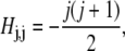 |
(11) |
|---|
and off-diagonal terms
 |
(12) |
|---|
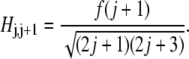
The vector of coefficients at point s is given by the matrix exponential of H:
 |
(13) |
|---|
This expression allows us to compute the probability distribution of the tangent vector orientation at any point along the chain. This result is exact if the infinite series of spherical harmonics is used. In practice, the series must be truncated for numerical calculations. Our calculations use N = 30 unless otherwise specified; the resulting truncation error is <0.1%.
The partition function is then calculated from the inner product
 |
(14) |
|---|
 |
(15) |
|---|
The extension at a given applied force is
 |
(16) |
|---|
This formula applies for a chain of any length.
Finite-length correction
To calculate the force-extension relation, we must determine M = _eℓ_H (Eq. 15). Because H includes at least one positive eigenvalue, the entries of M grow rapidly with ℓ. This increase can lead to numerical overflow errors when computing M. However, we are interested not in the entries of the matrix but in the logarithmic derivative of the partition function, and a rescaling can avoid the overflow problem.
Let A = _e_H and denote by λ* the largest eigenvalue of A. Then M = Aℓ. If we define  we have
  Thus 𝒜 has eigenvalues with magnitude ≤1. The partition function can be written as
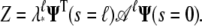 |
(17) |
|---|
The logarithm of the partition function is then
 |
(18) |
|---|
In the usual WLC solution, only the first term, an approximation which is exact in the limit  (4). The second term is the correction to ln Z due to finite-length effects.
Implementation of boundary conditions
The boundary conditions at s = 0 and s = ℓ affect the force-extension relation, because they affect the partition function (Eq. 15). The functional form of a specific boundary condition is given by the vector of coefficients Ψ(s = 0), which is determined by the projection of  onto spherical harmonics. To apply different boundary conditions, we simply determine the partition function for different vectors Ψ(s = 0) and Ψ(s = ℓ) (46).
In this article, we consider three types of boundary conditions (Fig. 4, A_–_C). First, in the unconstrained boundary conditions, the tangent vector at the end of the chain is free to point in any direction on the sphere (in 4_π_ of solid angle, Fig. 4 A). In real experiments, however, the boundary conditions are more constrained. If the polymer is attached to a surface about a freely rotating attachment point, we might expect half-constrained boundary conditions (Fig. 4 B) where the tangent vector at the end of the chain can point in any direction on the hemisphere outside the impenetrable surface. Half-constrained boundary conditions can be implemented experimentally with a flexible attachment between the chain and the surface (47). We also consider perpendicular boundary conditions where the tangent vector at the end of the chain is parallel to the  axis, normal to the surface (Fig. 4 C).
For the unconstrained boundary condition,  is independent of cos θ. Therefore
 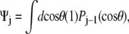 which gives Ψ = (1, 0, ···, 0). For the half-constrained boundary condition,
 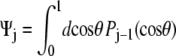 and the leading coefficients of Ψ are (1, 0.8660, 0, −0.3307, 0, 0.2073, 0). Finally, for the perpendicular boundary condition
 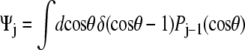 and the coefficients of Ψ are all equal to 1. (Note that for the computation of the force-extension relation, it is not necessary to properly normalize the probability distribution because we are computing the derivative of the logarithm of Z. Our expressions for the probability distribution vectors will neglect the constant normalization factor.)
In our results, we perform calculations for the one-bead and two-bead experimental geometries. In the first case, we assume that the s = 0 end of the chain is attached to the surface and the bead is attached at s = L.
Computation of bead rotational fluctuations
The bead rotational fluctuations lead to an effective boundary condition (at the end of the polymer) that depends on applied force and bead radius. For the single-bead experimental geometry (Fig. 2), Eq. 9 gives the partition function of the system including bead rotational fluctuations. We can perform the integral over  to find the probability distribution of
  which is the effective boundary condition at the end of the polymer. The integral over
  is
is
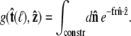 |
(19) |
|---|
Because the direction of  is constrained relative to the chain tangent
  this integral is a function of
  By azimuthal symmetry, it depends only on the scalar
  Accordingly, we can express Eq. 19 in the form
  where g is the probability distribution of tangent angles at s = ℓ. (Note that we neglect the normalization constant for g.) Expanding in spherical harmonics, we write
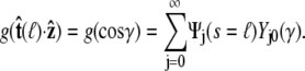 |
(20) |
|---|
The effective boundary condition depends on both the applied force and the radius of the bead. The physical characteristics of the polymer-bead attachment determine the constraints in the integral of Eq. 19 and therefore control the Ψj.
For the two-bead experimental geometry (Fig. 2 C), the partition function includes integrals over bead rotational fluctuations for both ends of the chain. Therefore, the effective boundary condition applies at both ends of the polymer.
Suppose that the polymer-bead attachment is half-constrained, so the tangent vector is free in a hemisphere (Fig. 4 B). Then the integral of Eq. 19 is constrained by  or
or
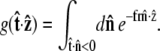 |
(21) |
|---|
To evaluate the integral, we choose a polar coordinate system where  points along the polar axis, and φ = 0 corresponds to the
  direction. Therefore
  and
and 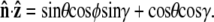 We can then write g in terms of the Bessel function _J_o.
 |
(22) |
|---|
 |
(23) |
|---|
 |
(24) |
|---|
Note that  and the integral from 0 to 2_π_ is even about π. We show some values of this function in Fig. 5 for different applied forces. As expected, for a small applied force and small bead radius, the probability distribution approaches a constant value (independent of cos γ). However, for a large applied force, the probability distribution approaches the half-constrained distribution one would expect in the absence of bead rotational fluctuations.
FIGURE 5.

Effective chain-end boundary conditions induced by bead rotational fluctuations. The unnormalized probability density  is shown versus
  for a bead of radius R = 250 nm. The different curves correspond to different values of the applied force. In this calculation, the attachment of the chain to the bead is half-constrained: in the absence of bead rotational fluctuations, the probability density is zero for cos γ < 0 and constant for cos _γ_ > 0. This step function is approached for a large force. For smaller values of FR, the probability density is smeared out and approaches a constant value (independent of cos γ).
Because cos θ is integrated over negative values in Eq. 24, the term e_−frcos_θ_cos_γ diverges as fr increases. However, we only calculate the dependence of g on cos γ (correct normalization is not required). Therefore we replace the term e_−frcos_θ_cos_γ in the integral with the term e_−fr(cos_θ_cos_γ+1). This is equivalent to multiplying the entire integral by _e_−fr, which does not vary with θ. Therefore, this rescaling does not change the dependence of g on γ.
To determine the effective boundary condition due to the rotationally fluctuating bead requires that we expand integrals of the form given in Eq. 24 in spherical harmonics. Direct numerical projection of the integral onto spherical harmonics leads to large errors because numerical integration of rapidly oscillating functions (such as the higher-order spherical harmonics) is inaccurate. To solve this problem, we used an interpolating basis (as in (48), section 3.1.4). This allows the coefficients of the spherical harmonics to be determined by evaluation of Eq. 24 at specific points (corresponding to the zeros of the Legendre polynomials). The integral in Eq. 24 was evaluated numerically using Gauss-Legendre quadrature.
The effective boundary condition due to bead rotational fluctuations is shown in Fig. 5 where we plot Eq. 24 for different values of the applied force; the curves are normalized so the curve lies between 0 and 1 and has a mean of 0.5. For a high applied force, rotational fluctuations require more energy and large-angle fluctuations are rare. Therefore, in the limit FR → ∞, the probability distribution approaches that of the chain-bead attachment (in this case, a step function). However, for smaller FR, the bead rotational fluctuations “smear out” the probability distribution, making the effective tangent-angle boundary condition approach a constant, independent of cos γ. For small FR, the boundary condition approximates the unconstrained boundary condition. For large FR, the effective boundary condition approaches the boundary condition that would occur with no bead.
FEATURES OF THE FWLC SOLUTION
FWLC predictions converge to WLC predictions as contour length increases
As expected, the FWLC predictions converge to the WLC predictions as the polymer contour length increases. Fig. 6 shows the predicted fractional extension x/L as a function of the chain contour length L (for fixed applied force). Predictions of the classic WLC solution are independent of contour length. However, for the FWLC, the predicted fractional extension deviates from the usual WLC prediction for smaller values of L/p. In all cases, the FWLC predictions converge to the classic WLC results as L/p → ∞.
FIGURE 6.

Convergence of the FWLC-predicted extension to the classic WLC prediction for large L. The predicted fractional extension x/L is shown as a function of the contour length L (at fixed applied force). The different curves correspond to different theoretical assumptions: 1), the classic WLC solution, calculated using the method of Marko and Siggia (4); 2), the FWLC with unconstrained boundary conditions at both ends of the chain; 3), the FWLC with half-constrained boundary conditions at both ends of the chain; and 4), the FWLC with perpendicular boundary conditions at both ends of the chain (see Fig. 4). The different panels show different applied forces: (A) 0.1 pN, (B) 1 pN. The polymer persistence length is p = 50 nm. Note that the WLC prediction is independent of contour length, and the FWLC predictions converge to the WLC prediction as L increases. The convergence occurs more quickly for higher applied force (note different y axis scales for different panels). For low applied force, the more constrained boundary conditions lead to a larger predicted fractional extension (see text).
Fitting FWLC curves to the classic WLC solution gives varying apparent persistence length
To develop intuition for the differences between the FWLC and the classic WLC solution, we fit predicted force-extension data (generated with the FWLC) to the WLC solution of Bouchiat et al. (26). We find that the contour length is typically fit well by the WLC solution, but a systematic error in the fitted value of the persistence length occurs (Fig. 7). The apparent persistence length decreases with contour length (Fig. 7 B) when bead rotational fluctuations are included in the solution, in a manner qualitatively consistent with our experimental observations.
FIGURE 7.

Results of fitting FWLC solution predictions to the classic WLC solution. The fitted value of the persistence length _p_∞ is shown as a function of contour length L. The polymer persistence length is p = 50 nm. (A) No bead. The different curves correspond to the unconstrained, half-constrained, and perpendicular boundary conditions at both ends of the chain. The apparent p decreases most for the half-constrained boundary conditions. The apparent persistence length decreases by >10 nm as L decreases from 105 to 100 nm. (B) One or two beads attached to the chain ends, with half-constrained boundary conditions at both ends of the chain.
We emphasize that our fitting result is not directly comparable to the fitting of experimental data because our simulated data are not noisy. However, the qualitative similarity in the apparent persistence length as a function of contour length suggests that the FWLC captures important physics for relatively short chains.
FWLC force-extension behavior depends on boundary conditions
We illustrate the force-extension curves for different boundary conditions and L/p = 10 in Fig. 8. The more the boundary conditions are constrained, the larger the deviations from the traditional WLC solution. The more constrained boundary conditions typically lead to a larger extension at low force. Therefore, the force-extension curves for the FWLC with unconstrained boundary conditions are closest to the classic WLC predictions.
FIGURE 8.

Force-extension curves predicted by the FWLC solution for L = 500 nm (L/p = 10) and different boundary conditions. The different curves correspond to the classic WLC solution and the FWLC with unconstrained, half-constrained, and perpendicular boundary conditions at both ends of the chain. The predicted extension for all boundary conditions converges at high force. For a low applied force <80 fN (shaded), the more constrained boundary conditions lead to a larger predicted extension, though our model may not adequately address steric interactions at these forces (see text).
We can use simple entropic arguments to understand the dependence of chain extension on boundary conditions. When the applied force is low, many different chain conformations are probable. Therefore, the boundary conditions and bead rotational fluctuations exert a greater influence on the chain extension. Unconstrained boundary conditions maximize the number of allowable conformations. In this case, the entropy is maximized, and the polymer extension is low; increasing the extension requires excluding many chain conformations, which requires more work. More-constrained boundary conditions restrict the number of conformations that are possible, leading to lower entropy and therefore a larger extension. At low force, the most constrained boundary conditions typically lead to the largest extension. We illustrate this idea with the limit of a perfectly rigid rod that is constrained at one end to be perpendicular to the surface. The infinite rigidity means that the molecule must be perfectly straight. The boundary conditions require that the polymer take only one conformation, perpendicular to the surface. In other words, the boundary conditions severely restrict the number of available conformations and thereby increase the predicted extension. (If the boundary conditions are unconstrained, the rod rotates to point in many different directions, and its average extension is lower).
Predicted force-extension behavior of a polymer attached to bead(s)
As discussed above and shown in Fig. 5, for small FR the boundary condition with a bead approaches the unconstrained boundary condition. This typically leads to a smaller extension than would occur in the absence of a bead. For large FR, the effective boundary condition approaches the boundary condition that would occur with no bead; therefore, there is little difference between the predicted extension with and without a bead at high applied force.
We note that two opposing trends occur as the bead radius varies. When the bead is smaller, the fractional error made by subtracting R from the measured extension to estimate the molecule extension is smaller, simply because one is subtracting a smaller value. However, for smaller R the restoring torque on the bead for a given F is also smaller, leading to larger angular fluctuations for smaller beads.
At very low forces, our FWLC solution gives inaccurate predictions, because it does not explicitly include the excluded-volume effects between the bead and the wall (49). If the force is very low, the predicted extension would imply that the bead overlaps with the wall (or the other bead). Typically we find that an applied force >80 fN is required to prevent predicted bead-wall overlap in our theory. Although the FWLC does lead to unphysical predictions at very low forces, the simple model of the bead rotational fluctuations is useful for larger values of the force.
RESULTS AND DISCUSSION
DNA elasticity analyzed with the WLC model
To determine limitations in the WLC solution for shorter chains, we systematically measured the elasticity of DNA for a broad range of DNA lengths (632–7030 nm) using an optical trap (Fig. 9). DNA molecules were attached to streptavidin-coated cover glass via biotin at one end and to an anti-digoxigenin-coated polystyrene bead via digoxigenin at the other end. We optically trapped the bead and moved the anchored end of the DNA relative to the optical trap using a three-axis closed-loop PZT stage (Fig. 1). We measured the resulting bead displacement _x_bd and force (_F_x = _k_trap_x_bd) as a function of distance _x_DNA along the x axis. Finally, we calculated the force F and the molecular extension x along the DNA axis based on the two-dimensional geometry (24). We fit each F versus x trace to an improved analytic approximation of the infinite WLC solution (26). This fit returns three values, _p_wlc, L, and Δ, where _p_wlc is the apparent persistence length, L is the contour length, and Δ is the location of the tether point (Fig. 9 A). We then repeated this procedure for many individual molecules at each length and for nine different length molecules ranging from 632 to 7030 nm.
FIGURE 9.

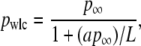
Experimental elasticity results. (A) Elasticity measurement of the 864-nm long DNA tether (magenta) stretched up to 8 pN in the positive and negative direction. A fit to the WLC solution (black) returns three values, _p_wlc, L, and Δ, where _p_wlc is the apparent persistence length, L is the contour length, and Δ is the location of the tether point. For the trace shown, the fitted values were 45.0 (±0.6) nm, −0.2 (±0.1) nm, and 863.0 (±0.4) nm, respectively. Data near the origin (1.2 R) are not used in the analysis due to experimental geometric constraints, where R is the radius of the trapped bead. (B) Force-versus-extension traces, with WLC fits, for a range of DNA lengths: 632 nm (lt. blue), 666 nm (lt. green), 756 nm (gold), 864 nm (magenta), 1007 nm (blue), 1514 nm (green), 2013 nm (orange), 2413 nm (purple), and 7030 nm (wine). Only the positive portion of the full records is shown for clarity. (C) Persistence length (mean ± SE) as a function of DNA length (top axis). The fit (green line) represents an empirical approximation to the experimental data over the range of DNA lengths studied where _p_wlc = _p_∞/(1 + a _p_∞/L), _p_∞ = 51.5 nm (dashed line) is the persistence length for an infinitely long DNA molecule, and a = 2.78. Extrapolation of this curve outside the experimentally tested length range is shown (dotted line). Since _p_wlc depends on L, we plot _p_wlc as a function of the number of persistence lengths (L/_p_∞) by using the length-independent _p_∞ (bottom axis).
Individual measurements of _p_wlc from different molecules of the same length showed significant variation (∼7%) that could mask any dependence of _p_wlc on L. We attribute the majority of this variation in _p_wlc to variations in the radius (R) of individual beads, not to differences in individual DNA molecules. Thus, individual measurements of _p_wlc at each length were averaged from more than 15 molecules; we report the mean and standard error of _p_wlc at each length.
Having averaged this random error in _p_wlc, our measurements revealed a substantial variation in the average value of _p_wlc with L (Fig. 9), referred to as _p_wlc hereafter for simplicity. For the longest chains studied (7030 nm), we measured _p_wlc to be 50.5 nm. Our determination of _p_wlc decreased by 8.5 nm or 17% for a DNA length of 632 nm. Indeed, the rate of decrease in _p_wlc increased with decreasing length (Fig. 9 C), suggesting that, for even shorter chains, this unphysical reduction in the persistence length would be even more severe.
We sought an analytic expression to capture the experimentally observed reduction in _p_wlc with L. Over the range of lengths measured, our data were well modeled by
 |
(25) |
|---|
with _p_∞ = 51.51 (±0.31) nm and a = 2.78 (±0.12), as shown in Fig. 9 C. This formula also enables us to determine a length-independent persistence length _p_∞, which is 1.0 nm larger than _p_wlc determined for L = 7030 nm. We caution that this experimental definition of _p_∞ is not based on a theoretical model, and the extrapolation to an infinitely long chain has not been experimentally tested for DNA molecules longer than L = 7030 nm. Nonetheless, it is desirable to have such a length-independent persistence length; we eliminate the ambiguity of which _p_wlc to use in calculating the number of persistence lengths in the molecule (L/p). Using this result, we also plot _p_wlc versus L/_p_∞ (Fig. 9 C), a dimensionless variable that quantifies the finite length of the chain in the statistically relevant parameter L/_p_∞ and provides a potential comparison between dsDNA and other macromolecules described by WLC solutions (28,29).
Dependence of _p_wlc on experimental parameters
Although our FWLC solution suggests a reduction in _p_wlc with decreasing L (Fig. 7), we looked for potential experimental artifacts that could cause this reduction (Fig. 10). First, we varied the minimum absolute force _F_min used in fitting the data. As shown in Fig. 9 A, we typically excluded the data closest to the origin due to limitations in the optical trapping geometry (24). This arbitrary minimum force did not affect our results (Fig. 10); _p_wlc for two different-length molecules (666 and 2413 nm) showed <1% variation for _F_min ≤ 0.6 pN. Thus, our determination of _p_wlc was robust to substantial changes in _F_min.
FIGURE 10.

Dependence of p_wlc on experimental parameters. (A) Percent variation in apparent persistence length (Δ_p/_p_0); mean ± SE) as a function of minimum force F_min used in fitting the data for two different DNA lengths, 666 nm (magenta) and 2413 nm (purple), where Δ_p = _p_0 – _p_F and _p_0 is the _p_wlc determined from fitting all of the data, and _p_F is the _p_wlc determined from the fit after excluding data below an absolute value _F_min in both the positive and negative directions. (B) Variation in persistence length (mean ± SE) as a function of the highest force (_F_max) used in fitting the data for two different DNA lengths, 666 nm (magenta) and 2413 nm (purple). A linear fit (dashed line) to the data yields a dependence of _p_wlc on _F_max of −1.8 nm/pN. (C) Persistence length (mean ± SE) as a function of DNA length at two different _F_max (6 and 8 pN) shows a systematic offset (as described in B). (D) The difference between the two traces in panel C shows a constant offset, suggesting the observed reduction of _p_wlc as a function of L is robust, although its absolute magnitude depends on _F_max.
Next, we varied the maximum force _F_max used in fitting the data. This arbitrary maximum force did affect our results (Fig. 10 B); two different length molecules (666 and 2413 nm) showed a systematic reduction in _p_wlc with increasing _F_max. The magnitude of the reduction for the two different lengths was similar, though with an offset. We quantified this reduction to be − 1.8 nm/pN by fitting _p_wlc for the 666-nm data to a line over the measured force range (4–8 pN). Additional data on a few DNA molecules stretched up to 12 pN suggest a continued linear decrease.
As the focus of this article is on the entropic stretching regime of DNA addressed by the WLC solution, we limited our maximum applied force to 8 pN. Above 8 pN, enthalpic stretching starts to become increasingly important (24). Yet, the standard WLC solution does not include enthalpic stretching, rather it computes entropic stretching, which at 8 pN of applied force leads to an extension of 95% of the contour length. Adding a stretch modulus, as is normally done (24), can lead to unphysically large persistence lengths unless the data are taken to quite high force. An auxiliary benefit of this moderate maximum force was that we were able to use smaller beads that in turn reduced the experimental geometric constraints.
To review the geometric constraints of the tethered particle in our optical trapping assay, a larger lateral displacement from the trap center leads to a larger vertical displacement (24). Small variations in _p_wlc with L could also arise from an incorrectly calibrated optical trap and/or an increasing vertical motion (_z_bd) of the trapped bead. While _z_bd is not directly measured, it is accounted for based on the experimental geometry. To address the first issue, we used a software-based position clamp (24) that varies the trap stiffness (_k_trap) to keep the bead (_x_bd) at a constant displacement (_x_clamp) from the trap center. Keeping the bead at a constant position reduces possible errors, including nonlinearity in the trapping force and incorrect position calibration. Yet, for this position clamp to be beneficial, the linearity of _k_trap with laser power _P_laser needs to be excellent. We assured this linearity in _k_trap by measuring and actively stabilizing the laser power (37). The position clamp was active over the force range of 1.2–8 pN. In addition, we sought to minimize _z_bd in the optical trap by setting _x_clamp = 40 nm to reduce other potential artifacts such as variation in _k_trap with _z_bd. Such an artifact might affect our results because _z_bd is dependent on the length of DNA studied; the angle θ increases as L decreases (Fig. 1). Thus it is noteworthy that measurements of _p_wlc at different _x_clamp did not change between _x_clamp = 30 and 40 nm over the range of lengths studied. This demonstrates that experimentally determined values of _p_wlc were robust and not due to a systematic variation in _p_wlc with L due to trapping geometry.
By reanalyzing all of our data with _F_max = 6 pN, we observed a systematic increase in _p_wlc versus _F_max for all DNA lengths measured (Fig. 10). However, the magnitude of this offset ( ) was fixed at ∼3 nm and did not depend on L (Fig. 10 D). Thus, our primary experimental observation of a reduction in _p_wlc with decreasing L does not depend on _F_max although the absolute magnitude of _p_wlc does.
While we did not experimentally change R, we theoretically investigated the effect of bead size. This analysis, based on elasticity data generated by our finite WLC solution that includes effects of bead size and rotational fluctuations, demonstrates that the predicted F versus x traces are insensitive to R over the valid force range (80 fN < F < 8 pN), as shown in Fig. 11. This experimental (Fig. 10) and theoretical analysis (Fig. 11), along with the aforementioned experimental procedures, suggest that our observed reduction in _p_wlc with decreasing L is real. Additionally, two complete, though initial data sets, taken at separate times using independent calibrations, yielded statistically indistinguishable results for the variation of _p_wlc with L.
FIGURE 11.

Force-extension curves predicted by the FWLC solution for L = 500 nm (L/p = 10) with one bead. We implemented half-constrained boundary conditions at both ends of the chain but included bead rotational fluctuations. The predicted molecular extensions, x (after the bead radius has been subtracted), agree with the no-bead prediction for large force, but decrease more rapidly as the force decreases. Such a reduction in x becomes more significant for bigger sized beads. The curves for two different beads (R = 100 and 250 nm) are indistinguishable over the theoretically valid force range (80 fN < F < 8 pN). Below 80 fN (shaded), the predicted x for a bead with R = 250 nm bead decreases faster than x for a bead with R = 100 nm.
Reduced dependence of p on L using the FWLC solution
Fitting our elasticity data to the WLC solution (Fig. 9 C) led to a systematic and unphysical reduction of p_wlc with L. Thus, we developed the finite wormlike chain (FWLC) solution by including three effects neglected in the classic (infinite chain) WLC solution: the finite length of the chain, boundary conditions, and bead rotation (see Theory). After incorporating these three corrections, we show that fitting experimental data to the FWLC solution reduced the dependence of p on L by threefold (Fig. 12). The fractional difference in Δ_p for the shortest molecules studied (632 nm) decreased from 18.3% to 6.8%, where Δ_p_ = _p_x − _p_∞ and _p_x is the persistence length determined using either the WLC or the FWLC solution (Fig. 12, red and blue, respectively). Thus, the FWLC solution provides a significantly improved theoretical framework in which to describe the elasticity of single DNA molecules over a broad range of experimentally accessible DNA lengths.
FIGURE 12.

Comparison between finite and classic (infinite chain) WLC solutions. (A) Persistence length determined by fitting experimental data to the classic WLC solution (_p_wlc, red) and the finite WLC solution using half-constrained boundary conditions (_p_fin, blue) as a function of DNA length. (B) Fractional error in the fitted p from _p_∞ showing an approximately threefold reduction in the length dependence of _p_fin as compared to _p_wlc. Ideally, p, an intrinsic property of the molecule, would be independent of L. Error bars represent the standard error of the mean.
CONCLUSIONS
We have experimentally demonstrated a significant limitation in the classic (infinite-chain) WLC solution. The persistence length, one of two required parameters for the WLC solution, is a material property related to bending stiffness, and it should not depend on length. Yet, for DNA molecules of even moderate length (L = 1300 nm, L/_p_∞ = 25), elasticity data analyzed with the classic WLC solution show an unphysical reduction of _p_wlc by 10%. Moreover, many recent single-molecule experiments use significantly shorter double-stranded nucleic acids because of the increased signal/noise ratio for resolving small, even 1 bp motion (25, 33). Our data show that analyzing shorter molecules with the classic WLC solution leads to unwanted systematic errors: the fractional error in _p_wlc rapidly increases with decreasing length.
Thus, we developed the finite wormlike chain (FWLC) solution to predict the elastic behavior of polymers over a broad range of experimentally accessible lengths, including short polymers (L/p ∼ 6–20). In addition to overcoming the standard assumption in the WLC solution—a very long polymer (L/_p_→∞)—our model incorporates two additional corrections to the WLC solution: 1), chain-end boundary conditions; and 2), bead rotational fluctuations. By fitting experimental elasticity data with the FWLC solution, we find a threefold reduction in the apparent decrease of p with L.
While this threefold improvement is significant and confirms that the FWLC incorporates the most important previously neglected physical effects, there is a still a small residual dependence of p on L. This discrepancy suggests the need to incorporate additional elements in future work beyond those already included in our model. For instance, in our experiments the DNA molecule is pulled at an angle θ relative to the surface (Fig. 1), though we theoretically model the DNA as being pulled vertically upward (Fig. 2 B). We also note that our FWLC solution is specialized for optical trapping assays. However, the general methodology developed here is immediately applicable to atomic force microscopy studies using dsDNA (50–53). In such experiments, analogous to our theoretical single-bead assay (Fig. 2 B), the boundary condition at the bead would be replaced by one compatible with an atomic force microscope tip; specifically, the tangent vector, confined to a half plane, is tilted at the tip's half cone angle with respect to the pulling direction.
Another class of potential physical effects becomes important at low forces, including the chain-chain, chain-wall, chain-bead, and bead-wall steric interactions. In our current calculations, we needed a force of ≈80 fN to keep the average position of the bead from physically overlapping with the coverslip. We expect such terms to be most important at very low (F < 100 fN) or zero applied force. Interpretation of zero-force experiments, such as the popular tethered particle assay, is becoming increasingly sophisticated; theoretical work shows the presence of a small, but nonzero entropic force (∼100 fN) that arises from bead-wall steric exclusion (49). This previously unrecognized force can alter kinetics of DNA looping (54). However, this theory uses the classic WLC solution to model and interpret experimental data (54). Our study shows that the use of the WLC solution may be a significant limitation, since most DNA looping experiments use short DNA molecules (L ≤ 300 nm) (55). Thus, we expect that incorporation of the FWLC into this existing formalism (49) will lead to further refinement in the interpretation of tethered particle data.
Our model makes an important testable prediction: the determination of _p_wlc with different trapping geometries should lead to different results. We report _p_wlc versus L for the widely used surface-coupled optical trapping assay where the DNA molecule is attached at one end to a bead (Fig. 1). We predict that similar experiments conducted with a dual-bead dual-trap assay should lead to an even larger unphysical decrease in _p_wlc with L than seen in our experiments (Fig. 2). This prediction highlights the importance of correctly modeling the whole experiment (Fig. 2, B and C) rather than simply modeling the elasticity of an isolated DNA pulled directly across its ends (Fig. 2 A).
In addition to the FWLC solution's improved description of the polymer elasticity, our model provides a clear answer to an important problem in experiments that use short polymers: the observed decrease in _p_wlc with L is neither a failure in experimental calibrations nor a result of multiple polymers attached to a single bead. Rather, it is a limitation in the infinite WLC solution. While a 50% decrease in _p_wlc is the hallmark of two side-by-side DNA molecules attached to a single bead, a 20% decrease was difficult to interpret. The origin of this decrease is now explained, and the experimentalist is free to study such a molecule with confidence.
In summary, the FWLC provides a single theoretical model to analyze single-molecule experiments over a broad range of experimentally accessible lengths. The FWLC will lead to more accurate and precise work with shorter polymers and thereby facilitate future discoveries in nucleic acid-enzyme interactions. Moreover, by elucidating the origin of a significant error in interpreting DNA elasticity (18% for L = 632 nm), our work should aid in the adoption of DNA as a molecular force standard (56).
Acknowledgments
The authors thank Wayne Halsey for DNA preparation, Igor Kulic, Rob Phillips, and Michael Woodside for useful discussions, and the Aspen Center for Physics and the Kavli Institute for Theoretical Physics, where parts of this work were done (M.D.B. and P.C.N.).
This work was supported by the Alfred P. Sloan Foundation (M.D.B.), a Burroughs Wellcome Fund Career Award in the Biomedical Sciences (T.T.P.), the Butcher Foundation (M.D.B., T.T.P.), a W. M. Keck Grant in the RNA Sciences (T.T.P.), National Institute of Standards and Technology (T.T.P.), and the National Science Foundation, grant No. Phy-0404286 (M.D.B., T.T.P.), grant No. Phy-0096822 (T.T.P.), grant No. DMR-0404674 (P.C.N.), and grant No. DMR-0425780 (P.C.N.). T.T.P. is a staff member of National Institute of Standards and Technology's Quantum Physics Division. Mention of commercial products is for information only; it does not imply NIST's recommendation or endorsement, nor does it imply that the products mentioned are necessarily the best available for the purpose.
Yeonee Seol and Jinyu Li contributed equally to this work.
Editor: Kathleen B. Hall.
References
- 1.Smith, S. B., L. Finzi, and C. Bustamante. 1992. Mechanical measurements of the elasticity of single DNA molecules by using magnetic beads. Science. 258:1122–1126. [DOI] [PubMed] [Google Scholar]
- 2.Bustamante, C., J. F. Marko, E. D. Siggia, and S. Smith. 1994. Entropic elasticity of _λ_-phage DNA. Science. 265:1599–1600. [DOI] [PubMed] [Google Scholar]
- 3.Perkins, T. T., S. R. Quake, D. E. Smith, and S. Chu. 1994. Relaxation of a single DNA molecule observed by optical microscopy. Science. 264:822. [DOI] [PubMed] [Google Scholar]
- 4.Marko, J. F., and E. D. Siggia. 1995. Stretching DNA. Macromolecules. 28:8759–8770. [Google Scholar]
- 5.Maier, B., D. Bensimon, and V. Croquette. 2000. Replication by a single DNA polymerase of a stretched single-stranded DNA. Proc. Natl. Acad. Sci. USA. 97:12002–12007. [DOI] [PMC free article] [PubMed] [Google Scholar]
- 6.Neuman, K. C., E. A. Abbondanzieri, R. Landick, J. Gelles, and S. M. Block. 2003. Ubiquitous transcriptional pausing is independent of RNA polymerase backtracking. Cell. 115:437–447. [DOI] [PubMed] [Google Scholar]
- 7.Wang, M. D., M. J. Schnitzer, H. Yin, R. Landick, J. Gelles, and S. M. Block. 1998. Force and velocity measured for single molecules of RNA polymerase. Science. 282:902–907. [DOI] [PubMed] [Google Scholar]
- 8.Wuite, G. J. L., S. B. Smith, M. Young, D. Keller, and C. Bustamante. 2000. Single-molecule studies of the effect of template tension on T7 DNA polymerase activity. Nature. 404:103–106. [DOI] [PubMed] [Google Scholar]
- 9.Yin, H., M. D. Wang, K. Svoboda, R. Landick, S. M. Block, and J. Gelles. 1995. Transcription against an applied force. Science. 270:1653–1657. [DOI] [PubMed] [Google Scholar]
- 10.Revyakin, A., R. H. Ebright, and T. R. Strick. 2004. Promoter unwinding and promoter clearance by RNA polymerase: detection by single-molecule DNA nanomanipulation. Proc. Natl. Acad. Sci. USA. 101:4776–4780. [DOI] [PMC free article] [PubMed] [Google Scholar]
- 11.Bianco, P. R., L. R. Brewer, M. Corzett, R. Balhorn, Y. Yeh, S. C. Kowalczykowski, and R. J. Baskin. 2001. Processive translocation and DNA unwinding by individual RecBCD enzyme molecules. Nature. 409:374–378. [DOI] [PubMed] [Google Scholar]
- 12.Perkins, T. T., H. W. Li, R. V. Dalal, J. Gelles, and S. M. Block. 2004. Forward and reverse motion of single RecBCD molecules on DNA. Biophys. J. 86:1640–1648. [DOI] [PMC free article] [PubMed] [Google Scholar]
- 13.Dumont, S., W. Cheng, V. Serebrov, R. K. Beran, I. T. Jr, A. M. Pyle, and C. Bustamante. 2006. RNA translocation and unwinding mechanism of HCV NS3 helicase and its coordination by ATP. Nature. 439:105–108. [DOI] [PMC free article] [PubMed] [Google Scholar]
- 14.Amit, R., O. Gileadi, and J. Stavans. 2004. Direct observation of RuvAB-catalyzed branch migration of single Holliday junctions. Proc. Natl. Acad. Sci. USA. 101:11605–11610. [DOI] [PMC free article] [PubMed] [Google Scholar]
- 15.Dawid, A., V. Croquette, M. Grigoriev, and F. Heslot. 2004. Single-molecule study of RuvAB-mediated Holliday-junction migration. Proc. Natl. Acad. Sci. USA. 101:11611–11616. [DOI] [PMC free article] [PubMed] [Google Scholar]
- 16.Dessinges, M. N., T. Lionnet, X. G. Xi, D. Bensimon, and V. Croquette. 2004. Single-molecule assay reveals strand switching and enhanced processivity of UvrD. Proc. Natl. Acad. Sci. USA. 101:6439–6444. [DOI] [PMC free article] [PubMed] [Google Scholar]
- 17.Smith, D. E., S. J. Tans, S. B. Smith, S. Grimes, D. L. Anderson, and C. Bustamante. 2001. The bacteriophage straight phi29 portal motor can package DNA against a large internal force. Nature. 413:748–752. [DOI] [PubMed] [Google Scholar]
- 18.Strick, T. R., V. Croquette, and D. Bensimon. 2000. Single-molecule analysis of DNA uncoiling by a type II topoisomerase. Nature. 404:901–904. [DOI] [PubMed] [Google Scholar]
- 19.Perkins, T. T., R. V. Dalal, P. G. Mitsis, and S. M. Block. 2003. Sequence-dependent pausing of single lambda exonuclease molecules. Science. 301:1914–1918. [DOI] [PMC free article] [PubMed] [Google Scholar]
- 20.van Oijen, A. M., P. C. Blainey, D. J. Crampton, C. C. Richardson, T. Ellenberger, and X. S. Xie. 2003. Single-molecule kinetics of lambda exonuclease reveal base dependence and dynamic disorder. Science. 301:1235–1238. [DOI] [PubMed] [Google Scholar]
- 21.van den Broek, B., M. C. Noom, and G. J. L. Wuite. 2005. DNA-tension dependence of restriction enzyme activity reveals mechanochemical properties of the reaction pathway. Nucleic Acids Res. 33:2676–2684. [DOI] [PMC free article] [PubMed] [Google Scholar]
- 22.Brower-Toland, B. D., C. L. Smith, R. C. Yeh, J. T. Lis, C. L. Peterson, and M. D. Wang. 2002. Mechanical disruption of individual nucleosomes reveals a reversible multistage release of DNA. Proc. Natl. Acad. Sci. USA. 99:1960–1965. [DOI] [PMC free article] [PubMed] [Google Scholar]
- 23.Bennink, M. L., S. H. Leuba, G. H. Leno, J. Zlatanova, B. G. de Grooth, and J. Greve. 2001. Unfolding individual nucleosomes by stretching single chromatin fibers with optical tweezers. Nat. Struct. Biol. 8:606–610. [DOI] [PubMed] [Google Scholar]
- 24.Wang, M. D., H. Yin, R. Landick, J. Gelles, and S. M. Block. 1997. Stretching DNA with optical tweezers. Biophys. J. 72:1335–1346. [DOI] [PMC free article] [PubMed] [Google Scholar]
- 25.Abbondanzieri, E. A., W. J. Greenleaf, J. W. Shaevitz, R. Landick, and S. M. Block. 2005. Direct observation of base-pair stepping by RNA polymerase. Nature. 438:460–465. [DOI] [PMC free article] [PubMed] [Google Scholar]
- 26.Bouchiat, C., M. D. Wang, J. F. Allemand, T. Strick, S. M. Block, and V. Croquette. 1999. Estimating the persistence length of a worm-like chain molecule from force-extension measurements. Biophys. J. 76:409–413. [DOI] [PMC free article] [PubMed] [Google Scholar]
- 27.Spakowitz, A., and Z.-G. Wang. 2004. Exact results for a semiflexible polymer chain in an aligning field. Macromolecules. 37:5814–5823. [Google Scholar]
- 28.Abels, J. A., F. Moreno-Herrero, T. van der Heijden, C. Dekker, and N. H. Dekker. 2005. Single-molecule measurements of the persistence length of double-stranded RNA. Biophys. J. 88:2737–2744. [DOI] [PMC free article] [PubMed] [Google Scholar]
- 29.Rief, M., M. Gautel, F. Oesterhelt, J. M. Fernandez, and H. E. Gaub. 1997. Reversible unfolding of individual titin immunoglobulin domains by AFM. Science. 276:1109. [DOI] [PubMed] [Google Scholar]
- 30.Hagerman, P. J. 1988. Flexibility of DNA. Annu. Rev. Biophys. Biophys. Chem. 17:265–286. [DOI] [PubMed] [Google Scholar]
- 31.Fixman, M., and J. Kovac. 1973. Polymer conformational statistics. 3. Modified Gaussian models of stiff chains. J. Chem. Phys. 58:1564–1568. [Google Scholar]
- 32.Liphardt, J., B. Onoa, S. B. Smith, I. Tinoco, and C. Bustamante. 2001. Reversible unfolding of single RNA molecules by mechanical force. Science. 292:733–737. [DOI] [PubMed] [Google Scholar]
- 33.Herbert, K. M., A. L. Porta, B. J. Wong, R. A. Mooney, K. C. Neuman, R. Landick, and S. M. Block. 2006. Sequence-resolved detection of pausing by single RNA polymerase molecules. Cell. 125:1083–1094. [DOI] [PMC free article] [PubMed] [Google Scholar]
- 34.Hori, Y., A. Prasad, and J. Kondev. 2007. Stretching short biopolymers by fields and forces. Phys. Rev. E. 75:041904. [DOI] [PubMed] [Google Scholar]
- 35.Kessler, D. A., and Y. Rabin. 2004. Distribution functions for filaments under tension. J. Chem. Phys. 121:1155–1164. [DOI] [PubMed] [Google Scholar]
- 36.Nugent-Glandorf, L., and T. T. Perkins. 2004. Measuring 0.1-nm motion in 1 ms in an optical microscope with differential back-focal-plane detection. Opt. Lett. 29:2611–2613. [DOI] [PubMed] [Google Scholar]
- 37.Carter, A. R., G. M. King, T. A. Ulrich, W. Halsey, D. Alchenberger, and T. T. Perkins. 2007. Stabilization of an optical microscope to 0.1 nm in three dimensions. Appl. Opt. 46:421–427. [DOI] [PubMed] [Google Scholar]
- 38.Visscher, K., S. P. Gross, and S. M. Block. 1996. Construction of multiple-beam optical traps with nanometer-resolution position sensing. IEEE J. Sel. Top. Quant. Electr. 2:1066–1076. [Google Scholar]
- 39.Neuman, K. C., E. A. Abbondanzieri, and S. M. Block. 2005. Measurement of the effective focal shift in an optical trap. Opt. Lett. 30:1318–1320. [DOI] [PMC free article] [PubMed] [Google Scholar]
- 40.Smith, S. B., Y. J. Cui, and C. Bustamante. 1996. Overstretching B-DNA: the elastic response of individual double-stranded and single-stranded DNA molecules. Science. 271:795–799. [DOI] [PubMed] [Google Scholar]
- 41.Storm, C., and P. C. Nelson. 2003. Theory of high-force DNA stretching and overstretching. Phys. Rev. E. 67:051906. [DOI] [PubMed] [Google Scholar]
- 42.Dhar, A., and D. Chaudhuri. 2002. Triple minima in the free energy of semiflexible polymers. Phys. Rev. Lett. 89:065502. [DOI] [PubMed] [Google Scholar]
- 43.Keller, D., D. Swigon, and C. Bustamante. 2003. Relating single-molecule measurements to thermodynamics. Biophys. J. 84:733–738. [DOI] [PMC free article] [PubMed] [Google Scholar]
- 44.Sinha, S., and J. Samuel. 2005. Inequivalence of statistical ensembles in single molecule measurements. Phys. Rev. E. 71:021104. [DOI] [PubMed] [Google Scholar]
- 45.Yamakawa, H. 1976. Statistical-mechanics of wormlike chains. Pure Appl. Chem. 46:135–141. [Google Scholar]
- 46.Samuel, J., and S. Sinha. 2002. Elasticity of semiflexible polymers. Phys. Rev. E. 66:050801. [DOI] [PubMed] [Google Scholar]
- 47.Nelson, P. C., C. Zurla, D. Brogioli, J. F. Beausang, L. Finzi, and D. Dunlap. 2006. Tethered particle motion as a diagnostic of DNA tether length. J. Phys. Chem. B. 110:17260–17267. [DOI] [PubMed] [Google Scholar]
- 48.Alpert, B., G. Beylkin, D. Gines, and L. Vozovoi. 2002. Adaptive solution of partial differential equations in multiwavelet bases. J. Comput. Phys. 182:149–190. [Google Scholar]
- 49.Segall, D. E., P. C. Nelson, and R. Phillips. 2006. Excluded-volume effects in tethered-particle experiments: bead size matters. Phys. Rev. Lett. 96:088306. [DOI] [PMC free article] [PubMed] [Google Scholar]
- 50.Clausen-Schaumann, H., M. Rief, C. Tolksdorf, and H. E. Gaub. 2000. Mechanical stability of single DNA molecules. Biophys. J. 78:1997–2007. [DOI] [PMC free article] [PubMed] [Google Scholar]
- 51.Rief, M., H. Clausen-Schaumann, and H. E. Gaub. 1999. Sequence-dependent mechanics of single DNA molecules. Nat. Struct. Mol. Biol. 6:346–349. [DOI] [PubMed] [Google Scholar]
- 52.Hansma, H. G., K. Kasuya, and E. Oroudjev. 2004. Atomic force microscopy imaging and pulling of nucleic acids. Curr. Opin. Struct. Biol. 14:380–385. [DOI] [PubMed] [Google Scholar]
- 53.Ke, C., Y. Jiang, M. Rivera, R. L. Clark, and P. E. Marszalek. 2007. Pulling geometry-induced errors in single molecule force spectroscopy measurements. Biophys. J. 92:L76–L78. [DOI] [PMC free article] [PubMed] [Google Scholar]
- 54.Blumberg, S., A. V. Tkachenko, and J. C. Meiners. 2005. Disruption of protein-mediated DNA looping by tension in the substrate DNA. Biophys. J. 88:1692–1701. [DOI] [PMC free article] [PubMed] [Google Scholar]
- 55.Finzi, L., and J. Gelles. 1995. Measurement of lactose repressor-mediated loop formation and breakdown in single DNA molecules. Science. 267:378–380. [DOI] [PubMed] [Google Scholar]
- 56.Rickgauer, J. P., D. N. Fuller, and D. E. Smith. 2006. DNA as a metrology standard for length and force measurements with optical tweezers. Biophys. J. 91:4253–4257. [DOI] [PMC free article] [PubMed] [Google Scholar]
- 57.Neumann, R. M. 1985. Nonequivalence of the stress and strain ensembles in describing polymer-chain elasticity. Phys. Rev. A 31:3516–3517. [DOI] [PubMed] [Google Scholar]