Quantitative Analysis of Isotope Distributions In Proteomic Mass Spectrometry Using Least-Squares Fourier Transform Convolution (original) (raw)
. Author manuscript; available in PMC: 2008 Aug 7.
Published in final edited form as: Anal Chem. 2008 Jun 4;80(13):4906–4917. doi: 10.1021/ac800080v
Abstract
Quantitative proteomic mass spectrometry involves comparison of the amplitudes of peaks resulting from different isotope labeling patterns, including fractional atomic labeling and fractional residue labeling. We have developed a general and flexible analytical treatment of the complex isotope distributions that arise in these experiments, using Fourier transform convolution to calculate labeled isotope distributions and least-squares for quantitative comparison with experimental peaks. The degree of fractional atomic and fractional residue labeling can be determined from experimental peaks at the same time as the integrated intensity of all of the isotopomers in the isotope distribution. The approach is illustrated using data with fractional 15N-labeling and fractional 13C-isoleucine labeling. The least-squares Fourier transform convolution approach can be applied to many types of quantitive proteomic data, including data from stable isotope labeling by amino acids in cell culture and pulse labeling experiments.
Stable isotope labeling in cells coupled with mass spectrometry has many important applications in the analysis of protein expression, modification, turnover, and metabolism.1 Cells and organisms can be isotopically labeled by supplying labeled precursors in the form of nutrients such as amino acids, glucose, and ammonia. These labeled precursors are incorporated into proteins, whose resulting isotope labeling patterns reflect their abundance and the dynamics of protein synthesis and turnover. The era of quantitative proteomics began with experiments where mixtures of unlabeled control cells and 15N-labeled or isotope depleted test cells were quantitatively analyzed to determine protein expression and phosphorylation levels.2,3 More recently, the SILAC technique was developed based on specific amino acid labeling of cells for quantitative analysis of protein expression, modification, and turnover.4–6
The two basic classes of quantitative metabolic labeling approaches are the stable isotope labeling by amino acids in cell culture (SILAC) experiments and pulse labeling experiments, both of which have been implemented in a variety of ways.7 In the SILAC method, independent samples are prepared with different labeling patterns that are mixed prior to mass spectrometry analysis. For pulse labeling experiments, labels that are added to the growth medium are taken up to metabolically label the proteome, which generates fractionally enriched proteins from a single sample. The isotopically labeled species in the latter of these two types of experiments have been produced either by atom-based labeling with a 15N-ammonia or a 13C-labeled carbon precursor in C. elegans, Drosophila,8 and Arabidopsis9 or by residue-based labeling with 15N-, 13C,- or 2H-labeled amino acids in Plasmodium.9 In both classes of experiments, quantitative comparison of the intensity of peaks from unlabeled and isotopically labeled peptides is an essential but complex and time-consuming step in the analysis of the resulting proteomic data.
One common complication in quantitative proteomic analysis is the occurrence of fractional isotope labeling due to the presence of unlabeled metabolites, resulting in complex iso-topomer distributions in the observed spectra.7 The growth of simple organisms on 15N-ammonium ions as the nitrogen source can result in fractional atom labeling of the proteins where the nitrogen atoms are composed of a statistical mixture of 14N and 15N atoms. The growth of more complex organisms on labeled amino acids can result in fractional residue labeling, where there is a statistical mixture of unlabeled and labeled residues. Most cellular labeling protocols are specifically adapted to maximize labeling extent and minimize metabolic scrambling to simplify the final data analysis. However, for experiments involving higher organisms, it can be difficult to achieve high isotopic enrichment in the required diet. For example, the metabolic labeling of chickens with feed containing 2H8-valine resulted in ~35% fractional residue labeling of valine residues, leading to complex isotope distributions for peptides containing multiple valine residues.10–12 A study of protein turnover in humans and rats achieved fractional atom labeling of only several percent by labeling with 2H2O.13 In contrast, metabolic labeling of C. elegans and Drosophila was achieved with a diet of 15N-labeled bacteria and yeast, respectively, resulting in ~95% fractional atom labeling of the entire organism with 15N.8 Even in this more favorable case, quantitative analysis of the resulting complex isotope distributions can be difficult.
Quantitation of peak amplitudes has been carried out by a variety of methods, including the use of monoisotopic peak heights and integration of peak areas. Quantitation of the extent of fractional atomic labeling is usually carried out by comparison of the experimental spectrum with a set of calculated isotope distributions.8,9,14–16 However, there are few general tools for the analysis of large data sets containing complex isotope distributions. Here, we have developed an analytical framework that provides a general solution to the quantitative analysis of arbitrarily complex isotope distributions. Fourier transform convolution provides a straightforward treatment of the isotope distributions of both fractional atom and fractional residue labeling. The relative abundance of species labeled with different isotope patterns can be determined at the same time as the extent of fractional atom labeling and fractional residue labeling. In combination with least-squares fitting to experimental data, this approach provides a quantitative method that is applicable to a wide variety of proteomic applications. The generality of the method is illustrated by quantitating the peptide peaks resulting from the fractional 15N-labeling and fractional amino acid labeling of 30S ribosomal proteins.
Calculation of Isotope Distributions in the _μ_-Domain
There are two basic approaches to the calculation of isotope distributions for species of high molecular weight and high isotopic complexity. The first is to explicitly evaluate the polynomial coefficients resulting from all the possible combinations of isotopes in the molecule. For large molecules, the polynomials have an extraordinary number of terms, and algorithms have been developed for truncating insignificant terms as the calculation progresses.17 This method is in widespread use, but the truncation can lead to distortions in the resulting isotope distributions and the results are not exact.18 The approach used here, originally developed by Rockwood, is to calculate isotope distributions exactly using Fourier transform convolution.18–20 There may be computational speed advantages to one or the other algorithm that depend on the molecular weight and number of points calculated, but current desktop computers can compute distributions for peptides in seconds or less. The Fourier transform (FT) convolution method used here requires no approximations and naturally lends itself to the computation of distributions from both fractional atom and fractional residue labeling, as described below.
Mass spectrometry data are recorded with intensity as the dependent variable and with the mass-to-charge ratio as the independent variable (the _m-_domain). A spectrum of N such points can be represented as S(mk), k = 0, 1, 2 … N. The mass spectrum has a conjugate Fourier representation as a frequency, s(μk), k = 0, 1, 2 … N, which is termed the _μ_-domain. The _m_-domain data are real-valued, while the _μ_-domain frequency representation is complex, and the two spectral representations can be intercon-verted by discrete forward Fourier transforms (FT) and inverse Fourier transforms (IFT), respectively.
| s(μ)=∑k=0N−1S(mk)exp(−2πi·mkμ/N) | (1) |
|---|
| S(m)=∑k=0N−1s(μk)exp(2πi·μkm/N) | (2) |
|---|
The intensity profile for a particular species can be calculated in the _μ_-domain prior to IFT by factoring s(μ) into three terms
where f(μ) contains the FT of the isotope distribution as a “stick” spectrum of infinitely sharp peaks, g(μ) is an instrumental line shape function, and h(μ) is a mass offset function. The isotope distribution function f(μ) is calculated as the product of the atomic isotope distributions fj(μ)
| f(μ)=∏j=1nelementsfj(μ)νj | (4) |
|---|
where _n_elements is the number of different elements in the molecule and νj is the number of atoms of type j in the molecule. The atomic isotope distribution functions Fj(m) are obtained by FT of the stick representation of the atomic isotope abundances
| Fj(m)=∑i=1njaijδ(m−mij)⇔fj(μ)=∑i=1njaijexp(2πi·mijμ) | (5) |
|---|
where nj is the number of isotopes for atom j, mij is the exact mass of isotope i for atom j, and aij is the fractional abundance of isotope i for atom j. The form for the instrument function g(μ) is usually taken to be a Gaussian. As described previously,19 it is computationally more efficient to move the spectrum toward the origin by a frequency shift in the _μ_-domain using a heterodyne function, which greatly reduces the number of points that must be calculated. The form for the heterodyne mass offset function is given by
where _m_hd is the heterodyne mass, or mass shift. The calculated _m_-domain spectrum S(m) obtained by IFT of s(μ) is shifted toward the origin by _m_hd. The form of eqs 1–6 is nearly identical to previously described treatments18–20 and provides a concise description of a mass spectrum in terms of the isotope distribution, the instrument function, and a mass offset.
In the present work, we apply and extend this analysis to compute isotope distributions commonly encountered in pro-teomic mass spectrometry experiments. First, a nonlinear least-squares method is implemented that provides fitted values for peak amplitudes as well as an explicit general treatment of the extent of fractional isotope labeling. Second, an alternative residue-based description of the isotope distribution function is developed that allows a general and flexible description of multiple labeled species with a combination of fractional residue labeling and fractional atomic labeling. The analysis of isotopomer distributions has many important applications in mass spectrometry, and the least-squares Fourier transform convolution (LS-FTC) approach described here facilitates the quantitative interpretation of complex isotope distributions.
EXPERIMENTAL PROCEDURES
Stable Isotope Pulse Labeling of E. coli
E. coli MRE600 (American type culture collection strain 29417), lacking ribonuclease I, was grown at 37 °C in M9 glucose minimal medium supplemented with trace metals and vitamins. For the 15N pulse experiments, the medium was prepared with 0.5 g/L 14N-ammonium sulfate as the sole nitrogen source. The cells were grown to OD600 0.5–0.6 and were then pulsed by the addition of 15N-ammonium sulfate solution directly to the culture, to a final concentration of 2.5 g/L. The culture was grown for an additional 100 min prior to harvest and ribosome preparation. For the 13C6-isoleucine and 2H10-leucine pulse experiments, the minimal medium was supplemented with all 20 amino acids, at concentrations of 1.5–105 mg/L. The concentrations of isoleucine and leucine were 14 and 21 mg/L, respectively. The cells were grown to ~OD600 0.6 and were then pulsed by adding the same amount of 13C6-isoleucine and/or 2H10-leucine, respectively. The culture was grown for an additional 30 min prior to harvest and ribosome preparation. Cell growth was stopped by adding crushed ice directly to the culture, followed by incubation for 20 min on ice and harvest by centrifugation at 6000 rpm for 10 min. Cells were stored at −80 °C.
Preparation of 30S Ribosomal Peptides
Frozen cell pellets were thawed and resuspended in Buffer A (20 mM Tris–HCl pH 7.5, 100 mM NH4Cl, 10 mM MgCl2, 0.5 mM EDTA, 6 mM β_-mercaptoethanol) and then lysed in a bead-beater (Biospec Products, Inc., Bartlesville, OK) using 0.1 mm zirconia/silica beads. Insoluble debris was removed by centrifugation at 31 000_g for 40 min. The supernatant was layered onto a 5 mL cushion of 1.1 M sucrose in Buffer B (20 mM Tris–HCl pH 7.5, 500 mM NH4Cl, 10 mM MgCl2, 6 mM _β_-mercaptoethanol), and the 70S ribosomes were pelleted by spinning at 37 200 rpm at 4 °C in a Ti 70.1 rotor (Beckman Coulter, Fullerton, CA) for 22 h. The supernatant was removed, the tube and 70S ribosome pellet were rinsed with Buffer C (50 mM Tris–HCl pH 7.8, 1 mM MgCl2, 100 mM NH4Cl, 6 mM _β_-mercaptoethanol), and the pellet was resuspended in Buffer C.
The 30S and 50S ribosomal subunits were dissociated at low [MgCl2] concentration (1 mM), and the subunits were separated on 36 mL gradients of 10–40% sucrose in Buffer C in a SW 32 rotor (Beckman Coulter, Fullerton, CA). The gradients were fractionated with a Brandel fractionator, and fractions containing 30S subunits were pooled and the proteins were precipitated by adding 100% w/v (6.1 N) trichloracetic acid (TCA) to 13% final concentration.21 Samples were incubated on ice for a minimum of 1 h, and for lower protein concentrations the incubation time was extended to overnight. The protein precipitates were pelleted by centrifugation at 16 000_g_ for 20 min at 4 °C. The supernatant was removed, and the pellets were rinsed first with ice-cold 10% TCA and then with ice-cold acetone.
The pellets were dried in a Speed-Vac concentrator and then resuspended in 20 _μ_L of 100 mM ammonium bicarbonate in 5% acetonitrile, then 2 _μ_L of 50 mM DTT was added, and the samples were incubated at 65 °C for 10 min. Cysteine residues were modified by the addition of 2 _μ_L of 100 mM iodoacetamide followed by incubation at 30 °C for 30 min in the dark. Proteolytic digestion of the 30S proteins was carried out by the addition of 2 _μ_L of 0.1 _μ_g/μ_L modified sequencing-grade porcine trypsin (Promega, Co., Madison, WI) with incubation overnight at 37 °C.21 To stop the digestion, formic acid was added to 0.1% final concentration, and the undigested protein precipitate was removed by centrifugation for 5 min at 20 000_g. An 8 _μ_L aliquot of the supernatant was used for the electrospray ionization time-of-flight (ESI-TOF) analysis.
ESI-TOF Mass Spectrometry
The peptide samples were analyzed on an Agilent 1100 Series high-performance liquid chromatography (HPLC) instrument coupled to an Agilent ESI-TOF instrument with capillary flow electrospray (Agilent Technologies, Inc., Santa Clara, CA). The samples (5–8 _μ_L) were injected using an autosampler onto an Agilent Zorbax SB C18 150 × 0.5 mm HPLC column. Peptides were separated on an aceto-nitrile (ACN) gradient in 0.1% formic acid at a flow rate of 7 _μ_L/min. The steps of the gradient were 5–15% ACN over 10 min, 15–47% ACN over 48 min, and 47–95% ACN over 4 min. Data were collected over the m/z range of 100–1300. A reference sprayer was used for some samples, which resulted in greater mass accuracy but slightly poorer signal.
Least-Squares Fitting of Peak Profiles
Two important features in the experimental spectrum must be accounted for to perform a least-squares fit to the data. First, the apparent mass in the spectrum is scaled by the inverse of the charge state of the ion. Second, application of the fast FT algorithm (FFT) requires uniform sampling in the m_-domain, and experimental spectra have slightly nonuniform sampling where Δ_m ∝ m.
The theoretical spectrum _S_calc(m) is calculated assuming unit charge, with mass as the independent variable. The independent variable for the experimental mass spectrum is the mass-to-charge ratio M = m/z, where z is the charge on the ion. For comparison with _S_calc(m), the experimental spectrum must be scaled according to the charge state z. It is straightforward to determine the charge state from the spacing of the peaks in the experimental isotope distribution, which is 1/z, giving the scaled spectrum
Alternatively the calculated spectrum could be scaled, but for least-squares fitting, scaling the experimental spectrum is done just once prior to fitting, while scaling the calculated spectrum would need to be done at each iteration.
The least-squares criterion for comparing a calculated and scaled spectra is given by the reduced _χ_-squared formula
| χ2=1nobs∑i=1nobs(Scalc(mi)−Sscale(mi))2σi2 | (8) |
|---|
where S_calc(mi), S_scale(mi), n_obs, and σi are the calculated spectrum, scaled experimental spectrum, number of points for comparison, and standard error for each point, respectively. In order to use the FFT algorithm for FT convolution, the spectrum must be approximated on a grid of uniformly sampled points with interval Δ_mc. For high-resolution spectra with Δ_m > 0.01 Da, it is generally sufficient to use Δ_mc = 0.001 Da. The calculated spectrum is computed over the interval of the peak profile, and for each point in _S_scale(m), the value of _S_calc(m) with the closest value of mi is used for each residual term in eq 8.
The most efficient least-squares minimization algorithms such as the Levenberg–Marquardt method22 take advantage of derivatives of the calculated function with respect to the fitting parameters. In addition, the use of derivatives can provide estimates of error for the fitted parameters by measuring the curvature of the _χ_2 surface at the minimum. Because the Fourier transform is a linear operation and because the form of eq 3 cleanly separates the fitting variables in the functions g(μ), h(μ), and f(μ), it is straightforward to differentiate _S_calc(m) with respect to the fitting parameters in the _μ_-domain prior to IFT. The expressions for derivatives of _χ_2 with respect to each of the parameters are given in the Supporting Information.
One potential benefit of the least-squares determination of parameters is that errors in the fitted parameters can be determined, provided that an independent and appropriate choice of σi can be made in eq 8. In practice this can be difficult, and experience has shown that the parameter errors from the fits tend to underestimate the true errors (data not shown). For this reason, we have adopted the practice of setting σi = 1 for least-squares fitting, and errors in the fitted parameters are determined by multiple independent observations.
Least-squares fitting was carried out using Levenberg–Marquardt minimization and FFT routines from Numerical Recipes in Fortran.23 The _μ_-domain functions were calculated using 32 768 complex points, providing 65 536 real points in the m_-domain, which corresponds to ~65 Da with a sampling of Δ_mc = 0.001 Da. The number of calculated points must be sufficient to contain the entire isotope distribution or spectral aliasing will occur, resulting in folding of the higher isotopomers into the lower part of the spectrum. The heterodyne mass shift was arbitrarily chosen to be 2–3 Da less than the monoisotopic mass for each peptide. Fitting was achieved using five rounds of Levenberg–Marquardt minimization, each with five iterations. During each round different parameters were allowed to vary, in a fitting schedule empirically determined to increase the convergence rate for large sets of peaks.
The radius of convergence depends heavily on the presence of interfering or overlapping peaks in the spectrum, and it is impossible to obtain a good fit in regions of severe spectral overlap. Convergence is also facilitated by starting with parameters in the neighborhood of the solution, which can be obtained either through knowledge of the labeling pattern or inspection of the raw peak profiles. Failure to converge is readily detected by large values of _χ_2 and nonsensical values of the fitted parameters, with convergence often obtained by selecting a different set of initial parameters. The quality of all fits is confirmed by visual inspection.
The sample data in Figure 1 are of high signal-to-noise ratio (~500:1), but the least-squares fitting is fairly robust for isolated peaks free from overlap. Although there is an inevitable decrease in accuracy with increasing noise, clean peaks such as those in Figure 1 can be analyzed with signal-to-noise ratios as low as 10:1. Least-squares fitting of the peak in Figure 1a performed on spectra with increasing amounts of added synthetic noise is available in the Supporting Information as Figure S1 and Table S1.
Figure 1.
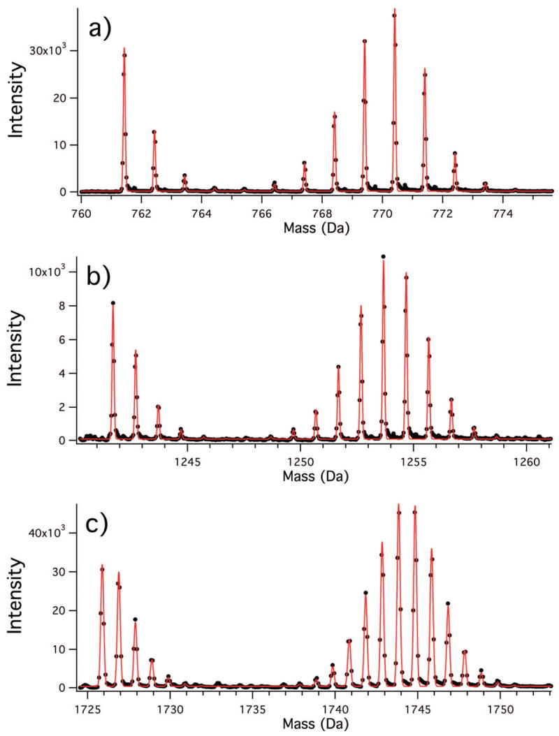
Composite peaks from unlabeled and fractionally 15N-labeled peptides resulting from pulse labeling. Experimental data points are shown as closed circles, and the least-squares fits using eqs 13–22 are shown as the solid line. (a) Protein S17 (residues 71–76), SWTLVR, z = 1. Fitted values: θ = 0.826, _f_L = 0.736. (b) S13(31–43), AILAAAGIAEDVK, z = 1. Fitted values: θ = 0.822, _f_L = 0.736. (c) S19(55–69), QHVPVFVTDEMVGHK, z = 4. Fitted values: θ = 0.826, _f_L = 0.737.
RESULTS
Vector Formalism for Calculation of Isotope Distributions in the _μ_-Domain
To facilitate the description of the μ_-domain functions below, a compact vector formalism is introduced here. For a given element j, the isotope abundances and exact masses can be expressed as column vectors **â_j**, and m̂j, respectively. For example, the abundance and mass vector for hydrogen are given by:
| a^1=[0.999850.00015]m^1=[1.007825042.01410179] | (9) |
|---|
The atomic μ_-domain isotope distribution functions can be conveniently expressed in terms of the vectors **â_j** and m̂j:
| fj(μ)=a^j·exp(2πiμm^j) | (10) |
|---|
The molecular formula for a peptide is expressed as _Hν_H_Cν_C_Nν_N_Oν_O_Sν_S, where the νj are the number of atoms of each type. The molecular formula can be equivalently expressed as vector n̂ of length _n_elements whose indices are the set of νj:
The set of atomic _μ_-domain functions can be similarly arranged into a vector F̂n(μ):
| F^n(μ)=[fH(μ)fC(μ)fN(μ)fO(μ)fS(μ)]T | (12) |
|---|
The _μ_-domain molecular isotope distribution function can be expressed in the compact form
| f(μ)=F^n(μ)n^=∏j=1nelementsfj(μ)νj | (13) |
|---|
where the exponentiation of the vector accumulates the product of the appropriate _μ_-domain functions, giving an equivalent expression to eq 4. These expressions give a compact formalism that will facilitate subsequent discussion of residue-based _μ_-domain functions.
Analytical Description of a Composite Unlabeled and Fractionally Labeled Isotope Distribution
Most quantitative applications in mass spectrometry involve the comparison of two peaks in a sample that have different isotope labeling patterns. For proteomic samples analyzed by LC-MS, this frequently involves quantitating the relative amount of 14N- and 15N-labeled peptides. In some cases, the exact isotopic composition of the labeled material may not be known or the goal may be to determine the fractional isotope enrichment, as in metabolic labeling and hydrogen–deuterium exchange experiments. A general fitting approach that handles fractional isotope enrichment and fractional residue labeling as fitting parameters would have many such applications.
In our laboratory, we have developed quantitative isotope pulse-chase assays to measure the assembly rates of 30S ribosomal proteins in vitro as they bind to 16S rRNA to form completed ribosomal subunits.24 In the course of extending the ribosome assembly work to metabolic labeling in rapidly growing E. coli, we encountered complex isotope distributions due to fractional 15N-labeling of peptides derived from ribosomal proteins. Consider the experimentally observed peaks shown in Figure 1, the mass spectrum of a peptide from bacterial cells that were treated with a pulse of 15N-ammonium sulfate for 100 min prior to harvesting the cells. The observed isotope distribution is the sum of the distributions from two distinct species. There is one isotope envelope from the unlabeled species present at the beginning of the 15N-pulse, and a second 15N-enriched isotope envelope from the species biosynthesized after the pulse. The observed spectrum can be expressed as the sum of the two isotope distributions for the two species
| Scalc(m)=B+AUSU(m)+ALSL(m) | (14) |
|---|
where B is a baseline offset, _A_U is the amplitude of the unlabeled distribution _S_U(m), and _A_L is the amplitude of the labeled distribution _S_L(m). The isotope distributions for the unlabeled and labeled species are readily calculated in the _μ_-domain:
In order to calculate the labeled distribution, a new atom type, N* for 15N-enriched atoms, is introduced for the labeled nitrogen atoms, and _n_elements is increased by one. The new vector of atomic _μ_-domain functions is given by:
| F^n(μ)=[fH(μ)fC(μ)fN(μ)fO(μ)fS(μ)fN∗(μ)]T | (17) |
|---|
The unlabeled part of the spectrum _S_U(m), is calculated using the _μ_-domain function _f_U(μ) calculated with the atomic composition vector n̂U
| fU(μ)=F^n(μ)n^Un^U=[νHνCνNνOνS0]T | (18) |
|---|
while the labeled part of the spectrum _S_L(m) is calculated using the _μ_-domain function _f_L(μ) calculated with the atomic composition vector n̂L:
| fL(μ)=F^n(μ)n^Ln^L=[νHνC0νOνSνN]T | (19) |
|---|
The exact mass vector for N* is identical to that of N, but the abundance vector for N* contains a new variable parameter θ that represents the fractional labeling with 15N:
The magnitude of the experimental error in the monoisotopic mass is expected to be on the order of the accuracy of the instrument, and for optimal peak fitting it is necessary to allow for small mass offsets due to calibration errors or limitations on accuracy. This small mass correction can be applied at the same time as the heterodyne mass shift, using a slightly modified form of eq 6
| h(μ)=exp(−2πi⋅μ(δm−mhd)) | (21) |
|---|
where _δ_m is a small mass correction offset (_δ_m ≪ 1).
Experimental peaks are well-approximated by a Gaussian shape, which can be obtained by convolution of the stick spectrum with a Gaussian function in the _μ_-domain:
| g(μ)=exp(−μ2/2γ2)2πγ | (22) |
|---|
This form of the Gaussian produces a unit-height peak irrespective of the width γ, which avoids covariation with the amplitude parameters during least-squares fitting.
These expressions provide an analytical description of a composite peak resulting from a natural abundance species and a fractionally 15N-labeled species. Thus, the composite peaks shown in Figure 1 can be completely described by six adjustable parameters: B, _A_U, _A_L, γ, _δ_m, and θ, given the molecular formula, exact masses, and isotope abundances. This in turn provides the possibility of quantitative analysis of the relative species abundance and the fractional labeling using least-squares fitting.
Least-Squares Fitting of Fractional 15N-Labeled Peaks
Analysis of isotope distributions is frequently performed by qualitative comparison of peak profiles with simulated distributions, or by correlation with a precomputed set of distributions.15 The goal of the present work is to quantitatively fit an experimental peak to a theoretical peak in the _m_-domain using a least-squares approach. Least-squares fitting can be accomplished by choosing an initial set of parameters and minimizing _χ_2 in eq 8 by iteratively calculating _S_calc(m) using eqs 14–22, while varying the parameters B, _A_U, _A_L, γ, _δ_m, and θ.
Least-squares fitting to the experimental peaks shown in Figure 1 gives excellent agreement. All of the essential features of the composite peaks are well-reproduced using the six-parameter description of the peak profile. The fractional 15N-labeling parameter θ is well-determined using least-squares fitting. At present, the errors in the fitted parameters are not obtained directly from the fits, but it is possible to determine the error empirically by analysis of a set of peptides from the same experiment. From the metabolic labeling experiment, a set of 291 peaks derived from 30S ribosomal peptides could be identified, in some cases from multiple charge states of the same peptide. An unsupervised least-squares fitting of these 291 peaks was carried out, and the value of θ was determined independently for each peak.
A histogram of the fitted values is shown in Figure 2A, with a box and whiskers plot at the top of the histogram. The average value is θ̄ = 0.825 ± 0.004, where the standard deviation is for the complete set of 291 fits. A majority of the fitted peaks give a tight clustering of θ, and there is a set of 23 clear outliers. Inspection of the individual spectra for the outliers revealed that the outlier values are primarily due to overlapping peaks that interfere with the fitting. A least-squares fit of the histogram of the entire set to a normal distribution gives θ = 0.825 ± 0.002. Clearly, the shape of the isotopomer profile is very sensitive to the extent of fractional labeling, and it is possible to precisely determine the value of θ to well within 0.2–0.3%. This is superior to the precision obtained by comparison with precalculated spectra (~1%),15 and the LS-FTC approach offers the advantage of a continuously varying adjustable parameter for fitting.
Figure 2.
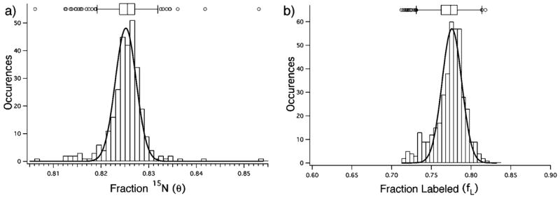
(a) Histogram of the distribution of the fractional labeling parameter (θ) determined by least-squares fitting for a set of 291 30S ribosomal peptides in a 15N-pulse labeling experiment. (b) Histogram of the distribution of the fraction labeled amplitude parameter (_f_L) determined by least-squares fitting for a set of 405 peptides derived from a 1:3 mixture of unlabeled and “100%” 15N-labeled 30S subunits. For both plots, a box-and-whiskers plot is shown at the top, indicating the median and the quartiles with boxes, and 1.5 times the interquartile range with whiskers. Clear outliers are indicated with open symbols at the top. For both plots, the normal distribution fitted to the entire set of values is shown as the solid line.
Of particular interest are the relative amplitudes of the unlabeled and labeled peaks, where the fraction of labeled peptide is given by:
Given that the doubling time of E. coli is ~40 min under these conditions, it would be expected that the fraction of newly labeled ribosomes would be on the order of ~0.8 in a 100 min pulse labeling experiment. The value of _f_L for the set of 291 fractionally labeled peaks is 0.74 ± 0.02, which shows that relative amplitudes can be determined with good precision. An additional experiment was performed on a known standard sample of unlabeled and fully 15N-labeled 30S ribosomes mixed in a 1:3 ratio. Least-squares fitting to a set of 406 peptides identified from an LC-MS data set was performed using eqs 14–22 as described for the pulse labeling experiment, except that the parameter θ was held fixed at a value of 0.993. A histogram of the calculated values of _f_L for the complete set of 406 peptides is shown in Figure 2B. The average value is _f_L = 0.77 ± 0.02, and a least-squares fit of the histogram to a normal distribution gives _f_L = 0.78 ± 0.02. These data demonstrate that relative quantitation of composite peaks from labeled and unlabeled samples can be accurately and precisely determined using the LS-FTC method.
Residue-Based Convolution of Isotope Distributions
Labeling with 15N-ammonium sulfate is useful for experiments with microorganisms, but in higher organisms it is often necessary to perform experiments with labeled amino acids in the growth medium. The LS-FTC method can be applied to these data, by expressing the molecular formula in terms of residue composition rather than atom composition. Residues, which each have their own predetermined atom composition, will usually be defined as amino acids, but any arbitrarily useful collection of atoms can be defined as a residue. A residue composition vector r̂j can be defined in analogy to n̂, whose elements give the atomic composition of that residue. The complete set of residue composition vectors can be assembled into a residue composition matrix:
| R∼=[r^1r^2…r^n_residues] | (24) |
|---|
The residue formula is given by a vector p̂ of length _n_residues, where the elements specify the number of each residue type in the species. The relationship between the molecular formula and residue formula is given by:
The _μ_-domain representation f(μ) can then be represented in the alternative residue basis
| f(μ)=F^n(μ)n^=F^n(μ)R^⋅p^=F^p(μ)p^ | (26) |
|---|
where
| F^p(μ)=F^n(μ)R∼=[F^n(μ)r^1F^n(μ)r^2…F^n(μ)r^n_residues]T=[fr^1(μ)fr^1(μ)…fr^n_residues(μ)]T | (27) |
|---|
Essentially the expressions in eqs 26 and 27 factor the _μ_-domain function in eq 4 according to residues instead of atoms. This new form allows for the incorporation of fractional residue labeling in calculation of isotope distributions.
Description of Fractional Residue Labeling
It is often impractical to achieve complete metabolic labeling with a stable-isotope-labeled amino acid. The ability to quantitatively describe fractional amino acid labeling will facilitate many types of metabolic labeling experiments. The residue _μ_-domain spectra in eq 27 are defined directly in terms of the molecular formulas for the amino acids. It can be useful to include an extra level of detail to treat the case where mixtures of different labeling patterns are present for a particular residue. For example, a mixture of unlabeled and 13C6-labeled isoleucine might be used for metabolic labeling, leading to a mixture of peptide isoto-pomers. In this case, the FT convolution can be used to facilitate the computation of the observed combinatorial mixtures. In analogy to the _μ_-domain expression for an atom as a linear combination of individual isotopes in eq 5, a residue can be defined as a linear combination of different labeling patterns:
| fj∗(μ)=Φ^⋅F^j∗Φ^=[1−φφ]F^j∗=[fj(μ)f'j(μ)] | (28) |
|---|
where φ is the residue fractional labeling parameter, which for the specific case of fractional 13C6-isoleucine labeling gives:
| fIle∗=(1−φ)fIle(μ)+φf13C6−Ile(μ) | (29) |
|---|
When multiple isoleucine residues are present in the peptide (_p_Ile > 1), the FT convolution implicitly and exactly calculates the combinatorial coefficients for the fractional labeling. This is carried out in the _μ_-domain in direct analogy to the combinatorials for the atomic isotope distributions by the expression fIle∗(μ)PIle.
An additional atom type, C* must be defined for the 13C-labeled atoms, and the residue compositions are given by:
which gives the following residue vectors for the unlabeled and labeled leucine residues, respectively:
The isotopic abundance for the C* atom is known in principle, but the enrichment given by suppliers is often approximate. It is straightforward to define a variable fractional 13C-enrichment in analogy to the fractional 15N-labeling described above. The abundance vector for the new fractionally labeled C* atom is specified as:
These expressions provide an analytical description of a combination of fractional residue and fractional atom labeling that can be used for least-squares fitting of fractionally labeled peptides.
Least-Squares Fitting for Fractional Residue and Fractional Atom Labeling
To prepare fractionally labeled peptides, rapidly growing E. coli were pulse-labeled with 13C6-isoleucine for 30 min. The starting medium contained 14 mg/L unlabeled isoleucine, and an equal amount of 13C6-isoleucine was added for the isotope pulse, which should produce fractional labeling in excess of 50%, depending on the amount of unlabeled isoleucine depleted from the medium by cell growth up to the time of the pulse. Ribosomes were isolated from these cells after a 30 min labeling period, and trypsin digests of the 30S ribosomal proteins were analyzed by LC-MS.
Representative peak profiles are shown in Figure 3 for the peptide ADIDYNTSEAHTTYGVIGVK, which corresponds to residues 179–198 from protein S3 in the +2 charge state, and for IVINQR, which corresponds to residues 27–32 of protein S9 in the +2 charge state. These peptides each contain two isoleucine residues, and the peak profile exhibits three expected groups of isotopomers at _m_0, _m_0+6, and _m_0+12, corresponding to peptides containing 0,1, and 2 labeled isoleucine residues, respectively.
Figure 3.
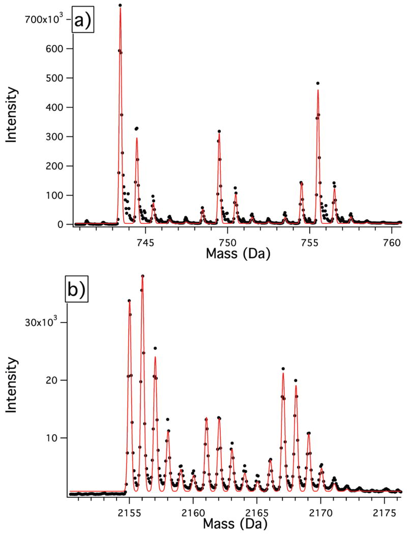
Composite peaks from unlabeled and fractionally 13C-Ile-labeled peptides resulting from pulse labeling. Experimental data points are shown as closed circles, and the least-squares fits using eqs 13–22 are shown as the solid line. (a) S9(27–32), IVINQR, z = 2. (b) S3(179–198), ADIDYNTSEAHTTYGVIGVK, z = 2.
The molecular formula for the +2 ion for S3(179–198) is (H146C94N24O34) which corresponds to the molecular formula vector
and the residue formula is A2D2EG2HI2KNST3V2Y2Z, where Z is the terminal residue for the atoms from the N- and C-termini, as well as the extra protons due to the net charge on the ion. The length of the residue composition vector is then augmented to 21 and has the value
| p^=[202102121001000132021] | (35) |
|---|
The peak profiles in Figure 3 are analytically described by the seven variable parameters B, _A_U, _A_L, γ, _δ_m, θ, and φ. The least-squares fit for the peak profiles are also shown in Figure 3, which shows excellent agreement with the experimental peak profile. The best fit values for the fractional 13C labeling (θ) of S3(179–198) and S9(27–32) are 0.976 and 0.974, respectively. The best fit values for the fractional isoleucine labeling are φ = 0.757 and φ = 0.759, respectively. These values are higher than the expected value (0.5) based on addition of 14 mg labeled isoleucine to medium containing 14 mg unlabeled isoleucine, which is due to the depletion of unlabeled isoleucine by cell growth prior to the isotope pulse.
The value of the fractional labeling parameter φ is effectively determined by the relative amplitude of the _m_0 + 6 and _m_0 + 12 peaks. The group of isotopomers at _m_0 contains contributions from both the unlabeled protein synthesized prior to the pulse and the fractionally labeled protein synthesized after the pulse. For the labeled species in Figure 3a, the fractional amplitudes of the _m_0, _m_0 + 6, and m_0 + 12 peaks for φ = 0.757 are (1 − φ)2 = 0.059, 2_φ (1 − φ) = 0.368, and _φ_2 = 0.573, respectively. The correct proportion of the _m_0 amplitude (0.059) for the labeled species is automatically included in the calculation of _A_L_S_L(m), and the value of _A_U adjusts during fitting to account for the remaining amplitude at _m_0. In the case where there is only one isoleucine residue in a given peptide, it is not possible to determine values for _A_L and φ independently, because the relative intensity of the _m_0 and _m_0 + 6 peaks depends both parameters in an anticorrelated way. In this case, the relative amount of labeled peptide can be determined by fixing φ = 1, but the contributions from before and after the pulse cannot be distinguished. However, once the value for φ has been determined for any one peptide from a protein, this value can be used to determine _A_L for other peptides from the same protein which can be assumed to have the same extent of fractional labeling.
In the LC-MS data set, eight peaks containing two or more isoleucine residues could be identified, and these arose from two different charge states for four distinct peptides, listed in Table 1. Least-squares fitting was performed for each of these peptides, and the complete set of fitted parameters is shown for each peptide in Table 1. The values of the fitted parameters that were determined independently for each peak agree extremely well. The average values and standard deviations are θ = 0.973 ± 0.006 and φ = 0.759 ± 0.014. The expected fractional 13C-enrichment was experimentally determined from the relative isotopomer peak heights in an ESI-TOF spectrum of the input 13C-isoleucine amino acid to be θ = 0.979, which is in good agreement with the values obtained from least-squares fitting of the peptide peak profiles. These results clearly demonstrate that the extent of fractional atomic and fractional residue labeling can be quantitatively extracted from peak profiles with excellent precision. In addition, the amplitudes of the labeled and unlabeled species are simultaneously determined, explicitly accounting for the overlapping contributions from these two species in the lowest mass isotope distribution.
Table 1.
Quantitation of Fractionally 13C.-Ile-Labeled Peptides
| peptide | sequence | m + _z_H | charge | θ (C*) | φ (13C-Ile) |
|---|---|---|---|---|---|
| S9(27-32) | IVINQR | 742.46 | 1 | 0.975 | 0.757 |
| S9(27-32) | IVINQR | 743.47 | 2 | 0.974 | 0.759 |
| S3(54-61) | IVIERPAK | 926.59 | 2 | 0.960 | 0.739 |
| S3(54-61) | IVIERPAK | 927.60 | 3 | 0.976 | 0.749 |
| S3(179-198) | ADIDYNTSEAHTTYGVIGVK | 2155.04 | 2 | 0.976 | 0.757 |
| S3(179-198) | ADIDYNTSEAHTTYGVIGVK | 2156.05 | 3 | 0.976 | 0.754 |
| S2(174-207) | EANNLGIPVFAIVDTNSDPDGVDFVIPGNDDAIR | 3571.76 | 3 | 0.970 | 0.769 |
| S2(174-207) | EANNLGIPVFAIVDTNSDPDGVDFVIPGNDDAIR | 3572.76 | 4 | 0.977 | 0.784 |
| avg | 0.973 | 0.759 | |||
| std dev | 0.006 | 0.014 |
Least-Squares Fitting for Double Fractional Residue Labeling
The residue-based description of the isotope distributions in the _μ_-domain makes it possible to analyze complex peak profiles, taking advantage of the FT convolution to directly compute the combinatorials for fractional residue labeling. To illustrate the power of this approach, a peak profile from a ribosomal peptide resulting from pulse labeling with 13C6-isoleucine and 2H10-leucine is shown in Figure 4. The sequence of this peptide is ISELSEGQIDTLRDEVAK, and the simultaneous fractional labeling of two isoleucine and two leucine residues produces a complex pattern in the isotope distribution.
Figure 4.
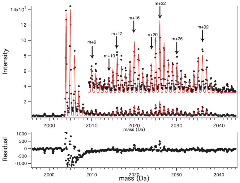
Composite peak from an unlabeled and fractional 13C-Ile/2H-Leu-labeled peptide resulting from pulse labeling. Experimental data points are shown as closed circles, and the least-squares fits using eqs 13–22 are shown as the solid line. The peptide sequence is ISELSEGQIDTLRDEVAK. The inset shows a vertical expansion of the fractionally labeled region. The main peaks resulting from the combinatorial residue labeling are indicated by arrows. The residuals from the fit, shown below, are dominated by the unlabeled peak, which has asymmetric tailing.
The residue-based formalism can be extended to treat this type of complex peak shape. Two fractional residue types are defined by
| fIle∗(μ)=(1−φIle)fIle(μ)+φIlef13C6−Ile(μ) | (36) |
|---|
| fLeu∗(μ)=(1−φLeu)fLeu(μ)+φLeuf2H10(μ) | (37) |
|---|
where _φ_Ile and _φ_Leu are the fractional labeling extents for isoleucine and leucine, respectively. Two labeled atom types, C* and H*, are introduced, and the residue formulas are expressed in terms of the augmented set of atoms:
| r^j=[νHνCνNνOνSνC∗νH∗] | (38) |
|---|
The abundance vectors for atoms C* and H* are given by
and the sum of the labeled and unlabeled contributions are given by eq 14 The complex peak shape shown in Figure 4 can be expressed in terms of the variable parameters B, A_U, A_L, γ, _δ_m, _θ_C, _θ_H, _φ_Ile, and _φ_Leu.
The successful least-squares fit to this peak profile is also shown in Figure 4, and the agreement is good. The basic features of this challenging isotope distribution are reproduced and can be understood in terms of the combinations of m + 6 and m + 10 for the two fractionally labeled residues. The residuals for the fit are also shown in Figure 4, which are largely due to an artifactual asymmetric feature at the base of the peaks in this spectrum. In this case, the quality of the information that can be quantitatively extracted from the peak is limited by the data itself, not the fitting process. It is clear that complex fractional atom and fractional residue labeling can be carried out using residue-based factoring of the _μ_-domain function and LS-FTC.
DISCUSSION
It is generally recognized that the quantitative analysis of fractional atomic and fractional residue labeling is a challenge for metabolic labeling experiments.7 The LS-FTC method described here provides a very general and flexible approach that can be adopted to facilitate the quantitation of many types of labeling experiments. A hierarchical definition is used for the multiple species present, the fractionally labeled residues, and the fractionally labeled atoms. The quantitative analysis of a particular data set can be customized for the particular labeling pattern chosen, and there is flexibility to control the number and nature of the adjustable parameters used.
Application to SILAC
This approach is particularly suited to quantitation of SILAC data from mixing of multiple samples with different labeling patterns. In a previous study, differential changes of the phosphotyrosine proteome upon the stimulation of mesenchymal stem cells with either platelet-derived growth factor or epidermal growth factor were monitored using different amino acids labels.25 The time dependence of the nucleolar proteome was studied using different amino acid labels for different time points.4 Both of these studies used unlabeled control cells and cells that had been labeled with either 13C6-arginine (Arg6) or 13C615N4-arginine (Arg10), resulting in isotope distributions with contributions from three species. It is straightforward to extend the LS-FTC approach to quantitate such data using the expression:
| Scalc(m)=B+AUSU(m)+AArg6SArg6(m)+AArg10SArg10(m) | (41) |
|---|
The LS-FTC approach would provide superior quantitation compared to using peak intensities, where the peak center may not lie directly on a sampled data point. The fitted amplitude parameters are determined from the entire peak profile, using all of the data points in the spectrum, and effectively integrating the intensity from all of the minor isotopomers.
A variety of alternative labeling strategies have been developed for absolute and relative quantitation in proteomics. Proteolytic labeling with H218O has been used effectively as a postlabeling technique for unlabeled tissues and specimens for quantitative comparison.27,28 ICAT29 and GIST30 are two widely used methods where peptides are chemically modified with reactive groups bearing isotope labels to provide relative quantitation between two samples. In addition, isotopically labeled peptides have been added as internal standards for quantitation, using synthetic labeled peptides in the AQUA approach31 or concatenated peptides expressed as labeled proteins in the QconCAT approach.32,33 All of these approaches generate isotope profiles that are composites from unlabeled and labeled species, and it straightforward to quantitate data from all of these methods using the LS-FTC approach described here.
Application to HDX
Hydrogen–deuterium exchange experiments are a powerful tool to study protein folding and dynamics. Analysis of HDX data requires determination of the extent of fractional deuterium labeling of hydrogen atoms that can exchange with solvent from the mass spectra of peptide fragments. There are three types of hydrogen atoms that contribute to the isotope distribution: nonexchangable aliphatic and aromatic hydrogen atoms, rapidly exchanging polar hydrogen atoms such as hydroxyls or carboxylates, and slowly exchanging hydrogen atoms primarily from the amide backbone. The residue formulas for the amino acids can be expressed as:
| r^j=[νCνNνOνSνHnonexνHfastνHslow] | (42) |
|---|
and the fractional labeling for the fast and slow exchanging hydrogens is given by the variable parameters _θ_fast and _θ_slow. The value of _θ_fast is typically determined from a control experiment, and the value of _θ_slow is the parameter of interest to be extracted from the peak profile. A variety of data analysis methods have been developed for HDX data, including the calculation of a centroid for the peak profile. An approach similar to LS-FTC was described previously for simultaneous identification and quantitation of HDX data using an atom-based description.34 More recently, an FT-deconvolution method has been reported for HDX data analysis,35 but in general deconvolution methods suffer from numerical instability, and the LS-FTC method offers the advantage of fitting the data in the domain in which it was acquired. In addition, a method that uses quantitative comparison with pre-calculated spectra to analyze HDX data has been reported.36 The LS-FTC method described here offers the advantage of a nonlinear least-squares quantitation using a small set of continuously adjustable parameters.
Application to Metabolic Labeling and Proteome Dynamics
Perhaps the most useful application for LS-FTC analysis of fractional atomic and fractional residue labeling will be studies carried out in plants and animals to monitor proteome dynamics. Analysis of data from the 15N-labeling of C. elegans and Drosophila8 can be carried out using the expressions in eqs 14–22. The extent of fractional 15N-labeling need not be known in advance and can be determined directly from the data simultaneously with the peak amplitudes. Furthermore, there is a reduced experimental requirement for complete labeling, since the isotope distribution for even 25% labeling can be cleanly resolved from the unlabeled distribution. We have shown that the extent of labeling can be precisely determined to within 0.2–0.3%.
The ability to interpret isotope distributions from partially labeled samples is particularly important for higher organisms. Expressions similar to eqs 28–33 can be used to treat data arising from fractional labeling of chicken muscle with 2H8-valine, which was achieved at levels of 35% from a diet containing 50% labeled valine. The complex isotope distributions in peptides containing multiple valine residues can readily be analyzed with LS-FTC to yield the extent of fractional labeling as well as the amplitudes of the labeled and unlabeled components. The time dependence of these amplitudes reveals information about protein synthesis and degradation rates in the animal.
A recent report on the labeling of Arabidopsis demonstrated that reliable quantitation can be obtained from partial 15N-labeling that compares well with the quantitation from full 15N-labeling.14 The approach to data analysis involves using ratios of isotopomers that are compared to precomputed distributions to determine the fractional labeling and to determine the relative amounts of each species. The LS-FTC method accomplishes both of these objectives by direct simulation of the experimental peak profile using a small number of adjustable parameters.
The LS-FTC method is extremely flexible and can readily be adapted to a large number of experimental systems. Computation of an isotope distribution with 65 000 points requires several seconds on a PowerPC G5 processor operating at 2.5 GHz, and least-squares fitting of a distribution can generally be accomplished with <30 iterations. The fitting is fairly robust in terms of convergence, since poor fits are readily detected by the _χ_2 value, and unconverged fits are readily detected by nonsensical values for the fitted parameters. The procedure has been automated for fitting of large data sets containing hundreds of peaks and integrated into the workflow of analysis of proteomic data.
CONCLUSIONS
The original use of FT convolution for calculation of isotope distributions was an elegant method developed for the simulation of isotope distributions.18–20 We have significantly extended this approach for the quantitative fitting of complex isotope distributions that arise in many types of proteomic mass spectra. A flexible and general framework for treating isotope distributions arising from combinations of species, from random fractional atom labeling, and fractional residue labeling was presented. Equivalent atom-based and residue-based representations of a molecular isotope distribution were developed, each with computational advantages for different labeling situations. This approach can easily be adapted for the quantitation of multiple species with different labeling patterns such as those that arise from SILAC experiments. Furthermore, because exact masses are used, the FT convolution can also be applied to high-resolution FT-MS and FT-ICR-MS data simply by increasing the resolution of the calculated spectra. The LS-FTC method presented here has numerous applications in quantitative mass spectrometry and provides a robust and flexible tool to treat complex isotope distributions observed for the molecular ions in high-resolution mass spectrometry.
Acknowledgments
This work was supported by grants from the NIH (R01-GM53757 to J.R.W. and F32-GM083510 to M.T.S.) and by The Skaggs Institute for Chemical Biology. The authors thank Stephen Chen for critical comments on the manuscript. The authors thank Drs. Gary Siuzdak and Sunia Trauger for many helpful discussions and for access to instrumentation at the TSRI Center for Mass Spectrometry.
Footnotes
SUPPORTING INFORMATION AVAILABLE Expressions for the derivatives of _χ_2 with respect to fitting parameters and Figure S-1 and Table S-1 describing the effects of noise on the fitting parameters. This material is available free of charge via the Internet at http://pubs.acs.org. The numerical calculations in this paper were carried out using the Fortran77 program isodist. The source code for isodist is freely available under the terms of the GNU General Public License at http://williamson.scripps.edu/software. Documentation and sample input and output data files from the figures in this paper are also available.
References
- 1.Smith JC, Lambert JP, Elisma F, Figeys D. Anal Chem. 2007;79:4325–4343. doi: 10.1021/ac070741j. [DOI] [PubMed] [Google Scholar]
- 2.Oda Y, Huang K, Cross FR, Cowburn D, Chait BT. Proc Natl Acad Sci USA. 1999;96:6591–6596. doi: 10.1073/pnas.96.12.6591. [DOI] [PMC free article] [PubMed] [Google Scholar]
- 3.Pasa-Tolic L, Jensen PK, Anderson GA, Lipton MS, Peden KK, Martinovic S, Tolic N, Bruce JE, Smith RD. J Am Chem Soc. 1999;121:7949–7950. [Google Scholar]
- 4.Andersen JS, Lam YW, Leung AKL, Ong SE, Lyon CE, Lamond AI, Mann M. Nature. 2005;433:77–83. doi: 10.1038/nature03207. [DOI] [PubMed] [Google Scholar]
- 5.Mann M. Nat Rev Mol Cell Biol. 2006;7:952–958. doi: 10.1038/nrm2067. [DOI] [PubMed] [Google Scholar]
- 6.Ong SE, Blagoev B, Kratchmarova I, Kristensen DB, Steen H, Pandey A, Mann M. Molecular & Cellular Proteomics. 2002;1:376–386. doi: 10.1074/mcp.m200025-mcp200. [DOI] [PubMed] [Google Scholar]
- 7.Beynon RJ, Pratt JM. Mol Cell Proteomics. 2005;4:857–872. doi: 10.1074/mcp.R400010-MCP200. [DOI] [PubMed] [Google Scholar]
- 8.Krijgsveld J, Ketting RF, Mahmoudi T, Johansen J, Artal-Sanz M, Verrijzer CP, Plasterk RHA, Heck AJR. Nat Biotechnol. 2003;21:927–931. doi: 10.1038/nbt848. [DOI] [PubMed] [Google Scholar]
- 9.Nelson CJ, Huttlin EL, Hegeman AD, Harms AC, Sussman MR. Proteomics. 2007;7:1279–1292. doi: 10.1002/pmic.200600832. [DOI] [PubMed] [Google Scholar]
- 10.Doherty MK, McLean L, Beynon RJ. Cytogenet Genome Res. 2007;117:358–369. doi: 10.1159/000103199. [DOI] [PubMed] [Google Scholar]
- 11.Doherty MK, Whitehead C, McCormack H, Gaskell SJ, Beynon RJ. Proteomics. 2005;5:522–533. doi: 10.1002/pmic.200400959. [DOI] [PubMed] [Google Scholar]
- 12.Hayter JR, Doherty MK, Whitehead C, McCormack H, Gaskell SJ, Beynon RJ. Mol Cell Proteomics. 2005;4:1370–1381. doi: 10.1074/mcp.M400138-MCP200. [DOI] [PubMed] [Google Scholar]
- 13.Busch R, Kim YK, Neese RA, Schade-Serin V, Collins M, Awada M, Gardner JL, Beysen C, Marino ME, Misell LM, Hellerstein MK. Biochim Biophys Acta. 2006;1760:730–744. doi: 10.1016/j.bbagen.2005.12.023. [DOI] [PubMed] [Google Scholar]
- 14.Huttlin EL, Hegeman AD, Harms AC, Sussman MR. Mol Cell Proteomics. 2007;6:860–881. doi: 10.1074/mcp.M600347-MCP200. [DOI] [PubMed] [Google Scholar]
- 15.MacCoss MJ, Wu CC, Matthews DE, Yates JR. Anal Chem. 2005;77:7646–7653. doi: 10.1021/ac0508393. [DOI] [PubMed] [Google Scholar]
- 16.Snijders APL, de Koning B, Wright PC. J Proteome Res. 2005;4:2185–2191. doi: 10.1021/pr050260l. [DOI] [PubMed] [Google Scholar]
- 17.Yergey J, Heller D, Hansen G, Cotter RJ, Fenselau C. Anal Chem. 1983;55:353–356. [Google Scholar]
- 18.Rockwood AL, Vanorden SL, Smith RD. Anal Chem. 1995;67:2699–2704. [Google Scholar]
- 19.Rockwood AL. Rapid Commun Mass Spectrom. 1995;9:103–105. [Google Scholar]
- 20.Rockwood AL, VanOrden SL. Anal Chem. 1996;68:2027–2030. doi: 10.1021/ac951158i. [DOI] [PubMed] [Google Scholar]
- 21.Link AJ, Fleischer TC, Weaver CM, Gerbasi VR, Jennings JL. Methods. 2005;35:274–290. doi: 10.1016/j.ymeth.2004.08.019. [DOI] [PubMed] [Google Scholar]
- 22.Marquardt DW. J Soc Ind Appl Math. 1963;11:431–441. [Google Scholar]
- 23.Press WH, Teukolsky SA, Vetterling WT, Flannery BP. Numerical Recipes in Fortran 77: The Art of Scientific Computing. Cambridge University Press; Cambridge: 2001. [Google Scholar]
- 24.Talkington MWT, Siuzdak G, Williamson JR. Nature. 2005;438:628–632. doi: 10.1038/nature04261. [DOI] [PMC free article] [PubMed] [Google Scholar]
- 25.Kratchmarova I, Blagoev B, Haack-Sorensen M, Kassem M, Mann M. Science. 2005;308:1472–1477. doi: 10.1126/science.1107627. [DOI] [PubMed] [Google Scholar]
- 26.Fenselau CJ. Chromatogr B: Anal Technol Biomed Life Sci. 2007;855:14–20. doi: 10.1016/j.jchromb.2006.10.071. [DOI] [PubMed] [Google Scholar]
- 27.Yao XD, Afonso C, Fenselau C. J Proteome Res. 2003;2:147–152. doi: 10.1021/pr025572s. [DOI] [PubMed] [Google Scholar]
- 28.Yao XD, Freas A, Ramirez J, Demirev PA, Fenselau C. Anal Chem. 2004;76:2675–2675. [Google Scholar]
- 29.Gygi SP, Rist B, Gerber SA, Turecek F, Gelb MH, Aebersold R. Nat Biotechnol. 1999;17:994–999. doi: 10.1038/13690. [DOI] [PubMed] [Google Scholar]
- 30.Chakraborty A, Regnier FE. J Chromatogr, A. 2002;949:173–184. doi: 10.1016/s0021-9673(02)00047-x. [DOI] [PubMed] [Google Scholar]
- 31.Gerber SA, Rush J, Stemman O, Kirschner MW, Gygi SP. Proc Natl Acad Sci USA. 2003;100:6940–6945. doi: 10.1073/pnas.0832254100. [DOI] [PMC free article] [PubMed] [Google Scholar]
- 32.Pratt JM, Simpson DM, Doherty MK, Rivers J, Gaskell SJ, Beynon RJ. Nature Protocols. 2006;1:1029–1043. doi: 10.1038/nprot.2006.129. [DOI] [PubMed] [Google Scholar]
- 33.Rivers J, Simpson DM, Robertson DHL, Gaskell SJ, Beynon RJ. Mol Cell Proteomics. 2007;6:1416–1427. doi: 10.1074/mcp.M600456-MCP200. [DOI] [PubMed] [Google Scholar]
- 34.Palmblad M, Buijs J, Hakansson P. J Am Soc Mass Spectrom. 2001;12:1153–1162. doi: 10.1016/S1044-0305(01)00301-4. [DOI] [PubMed] [Google Scholar]
- 35.Hotchko M, Anand GS, Komives EA, Ten Eyck LF. Protein Sci. 2006;15:583–601. doi: 10.1110/ps.051774906. [DOI] [PMC free article] [PubMed] [Google Scholar]
- 36.Pascal BD, Chalmers MJ, Busby SA, Mader CC, Southern MR, Tsinoremas NF, Griffin PR. BMC Bioinformatics. 2007;8:156. doi: 10.1186/1471-2105-8-156. [DOI] [PMC free article] [PubMed] [Google Scholar]