Correcting Estimators of θ and Tajima's D for Ascertainment Biases Caused by the Single-Nucleotide Polymorphism Discovery Process (original) (raw)
Abstract
Most single-nucleotide polymorphism (SNP) data suffer from an ascertainment bias caused by the process of SNP discovery followed by SNP genotyping. The final genotyped data are biased toward an excess of common alleles compared to directly sequenced data, making standard genetic methods of analysis inapplicable to this type of data. We here derive corrected estimators of the fundamental population genetic parameter θ = 4_N_e_μ_ (_N_e, effective population size; μ, mutation rate) on the basis of the average number of pairwise differences and on the basis of the number of segregating sites. We also derive the variances and covariances of these estimators and provide a corrected version of Tajima's D statistic. We reanalyze a human genomewide SNP data set and find substantial differences in the results with or without ascertainment bias correction.
THE HapMap data (International HapMap Consortium 2007) and other genomewide single-nucleotide polymorphism (SNP) data sets provide a valuable resource for population genetic analysis. Much interest in the analysis of such data has focused on estimating demographic parameters or inferring natural selection (e.g., Bamshad and Wooding 2003; Wooding 2004; Carlson et al. 2006; Sabeti et al. 2006; Voight et al. 2006; Wang et al. 2006; Tang et al. 2007; Williamson et al. 2007). However, many of the studies of genomewide SNP data have been challenged by the fact that the SNP genotyping data have been obtained by a process in which SNPs are first discovered in a small panel of individuals and subsequently typed in a much larger panel (e.g., Picoult-Newberg et al. 1999; Altshuler et al. 2000; Mead et al. 2003). Although this procedure provides a much faster and cheaper way of generating data than direct sequencing of the full panel, it also produces data with a relative excess of alleles of intermediate frequencies compared to directly sequenced data. Rare SNPs are more easily discovered in large panels than in small panels, so an initial discovery process based on a small panel produces an excess of high-frequency alleles in the genotyped sample. As a consequence, the data will be different from what is assumed in standard population genetic models with respect to allele frequency distribution (e.g., Nielsen 2000; Wakeley et al. 2001), patterns of linkage disequilibrium (Nielsen and Signorovitch 2003), and level of population subdivision (Nielsen 2004). This ascertainment bias toward high-frequency alleles can have serious consequences when standard population genetic tools (e.g., Tajima 1989; Fu and Li 1993; Fay and Wu 2000; Ramos-Onsins and Rozas 2002) are used for the analysis of the data. For example, Kreitman and Di Rienzo (2004) and Soldevila et al. (2005) showed that the apparent effects of balancing selection detected in the prion protein gene (PRPN) by Mead et al. (2003) in fact were an artifact caused by this type of ascertainment bias.
Three different approaches have been used to address the problem of ascertainment biases in studies of real data: (i) applying methods that may be more robust to the effect of ascertainment bias, such as methods based on haplotype structure (e.g., Sabeti et al. 2002), (ii) simulating data under the ascertainment procedure to derive appropriate critical values and confidence intervals using a distribution that directly takes ascertainment into account (e.g., Carlson et al. 2004; Voight et al. 2006), and (iii) directly correcting the statistical estimators and statistics for the ascertainment bias (e.g., Nielsen 2000; Wakeley et al. 2001; Nielsen and Signorovitch 2003; Polanski and Kimmel 2003; Marth et al. 2004; Nielsen et al. 2004) in specific models. However, hitherto there have been no ascertainment correction methods available for some of the most basic population genetic tools. Here we derive ascertainment corrected estimators of the fundamental population genetic parameter θ = 4_N_e_μ_ (_N_e, effective population size; μ, mutation rate) and an ascertainment corrected version of the popular statistic used for detecting selection: Tajima's D. Our results are for a neutral locus, without recombination, sampled from a panmictic population of constant size.
THEORY AND METHODS
Estimators of θ:
Tajima's D (Tajima 1989) is calculated as the difference between Tajima's estimator of θ, θT (Tajima 1989), and Watterson's estimator of θ, θw (Watterson 1975). Tajima's estimator is based on the average number of pairwise differences (π) and is given by
 |
(1) |
|---|
where η_i_ is the number of derived alleles segregating at a frequency of i/n, in a sample of n chromosomes. The calculation of  is identical for arbitrarily labeled alleles; however, we use the definition on the basis of knowing which allele is derived, to keep a consistent notation throughout. Watterson's estimator is given by
 |
(2) |
|---|
where  is the number of segregating sites.
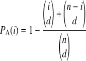
We assume an ascertainment model in which a subset of d chromosomes has been chosen independently among the n chromosomes for ascertainment, as the data to be analyzed later are the result of this same discovery procedure. We further assume that the chromosomes chosen for ascertainment are independent among SNPs; that is, each SNP has been ascertained from a different set of chromosomes. This procedures simulates the data obtained from procedures such as shotgun or array-based resequencing (used in Perlegen data), where different individuals are sequenced and the fragments obtained are aligned using a reference sequence. The probability of ascertainment of a SNP with alleles of frequencies i/n and (n − i)/n is then
 |
(3) |
|---|
(Nielsen 2004), where we use the definition  if k > n. The final sample after ascertainment is denoted the genotyped sample.
The expected number of segregating sites in the genotyped sample under this ascertainment scheme, S(A), is then simply the sum over all allelic classes of the expected number of segregating sites of that allelic class (_E_[η_i_] = θ/i; Tajima 1989; Fu 1995) multiplied by the probability of ascertainment of the allelic class:
 |
(4) |
|---|
An unbiased, ascertainment corrected method-of-moments estimator of θ, similar to Watterson's estimator, is then given by
 |
(5) |
|---|
The expected number of pairwise differences in the genotyped sample is similarly given by the sum over all allelic classes of the expected contribution to the pairwise differences of the allelic class multiplied by the probability of ascertainment of the allelic class:
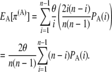 |
(6) |
|---|
An unbiased, ascertainment corrected method-of-moments estimator similar to Tajima's estimator is then given by
 |
(7) |
|---|
Note that these estimators are identical to the traditional estimators,  and
and  , when there is no ascertainment bias; i.e.,
  .
.
Variances of the estimators:
We use notation and some results from Durrett (2008, Chap. 2), to derive covariance and variances of these estimators assuming no intralocus recombination. In the absence of any ascertainment bias (Fu 1995; Durrett 2008),

where  equals
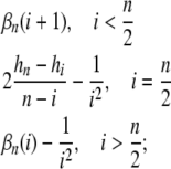 |
(8) |
|---|
 equals
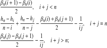
and

Using the conditional variance formula
 |
(9) |
|---|
with  and
and  , we get
 |
(10) |
|---|
Also, from Equation 8 and from the independence among SNPs of the ascertainment probabilities, we have

Then, recalling that  , we obtain
 |
(11) |
|---|
We can then easily get the variance of S(A):
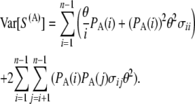 |
(12) |
|---|
The variance of the ascertainment corrected estimator of θ based on the number of segregating sites is then given by
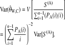 |
(13) |
|---|
The variance of the estimator based on the average number of pairwise differences becomes
 |
(14) |
|---|
Covariances and Tajima's D:
Defining the coefficients

we have
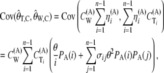 |
(15) |
|---|
by using Equations 10 and 11 and expanding the covariance of the sums as the sum of the covariances.
Also
 |
(16) |
|---|
We now define an ascertainment corrected Tajima's D as
 |
(17) |
|---|
To calculate  for real data we need to know the value of θ and θ2. We estimate θ using
  , similarly to the usual use of
  for calculating the classical Tajima's D statistic. We estimate θ2 as
 |
(18) |
|---|
The _D_C statistic is identical to the traditional Tajima's D in the absence of an ascertainment, i.e., when  .
.
Simulations:
Simulated data were generated using the standard coalescent simulation program ms (Hudson 2002) with 10,000 and/or 1,000,000 replicates. We explored three different values of θ: 2.23, 22.33, and 89.30, corresponding to the estimates of θ based on Watterson's estimator calculated from the minimum, average, and maximum number of segregating sites found in the genes represented in the SeattleSNP database (http://pga.gs.washington.edu/, Crawford et al. 2005). We also explored results for an extreme value of θ, θ = 150. To generate ascertainment samples from the simulated data, we subsampled d (= 2, 5, or 10) gene copies from each segregating site in the sample of size n (= 20 or 50). Moreover, we have also generated a set of samples of size n = 100 to explore the relationship between d and the variance in the estimators. If the segregating site was polymorphic in the subsample, it was included in the final sample; otherwise it was ignored. In all cases, the recombination rate was set to 0.
Perlegen data:
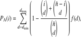
Genotype data from Perlegen were obtained from http://genome.perlegen.com/browser/download.html, and we used information regarding the ascertainment protocol discussed in Clark et al. (2005) and Hinds et al. (2005). For each SNP, the number of individuals that have been included in the discovery panel is known for 69% of the SNPs (ascertainment panel A), and only these SNPs are included in our analysis. Ascertainment of SNPs in this panel was done by genomewide shotgun resequencing. Data from all populations were pooled, and Tajima's D was calculated chromosome by chromosome through a sliding window of 100 and 500 kb, sliding by 10 kb at a time. To take into account varying sample size (n) and varying ascertainment sample size (d), for each window, we use
 |
(19) |
|---|
where  is the average sample size in the window, f(d) is the proportion of SNPs with ascertainment sample size d, and _d_max and _d_min are the maximal and minimal values of d observed in the window. We use this approach instead of a SNP-by-SNP correction to reduce the computational complexity of the problem. Only those windows that contained at least 10 class A SNPs were included in the analysis. To examine the effect of the ascertainment bias, we have included results for both the uncorrected and the corrected values of Tajima's D.
RESULTS
We evaluate the corrections of  and
and  , their variances and covariances, and Tajima's D using coalescent simulations in the first three subsections. Subsequently, we apply the corrected Tajima's D on the Perlegen data set.
Correction of the estimators of θ:
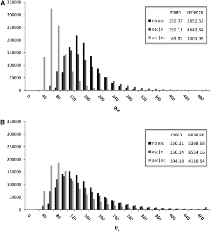
Figure 1 shows the distribution of the estimates based on the uncorrected estimators  and
and  , in the presence of an ascertainment bias (d = 5) and without an ascertainment bias (d = n = 50), and the corresponding distributions of the corrected estimates,
  and
and  , in the presence of an ascertainment bias for n = 50 and θ = 150. For
  , the average estimate of θ is 69.82 with and 150.07 without an ascertainment bias, respectively. However, the ascertainment corrected estimate is
  = 150.11. For
  , the average estimate of θ is 104.18 with and 150.11 without an ascertainment bias, respectively, and the ascertainment corrected estimate is
  = 150.14. For θ = (2.23, 22.33, and 89.20) we also found large differences between the average estimates of θ with and without an ascertainment bias, while the true value was recovered under ascertainment when the corrected estimators were used (see supplemental data A for more details). This shows that the traditional estimators, as expected, are biased in the presence of an ascertainment bias, but that the ascertainment corrected estimators derived here recover an unbiased estimate.
Figure 1.—
The distribution of the estimates of θ assuming nonascertained data (no asc), ascertained data with correction (asc | c), and ascertained data without correction (asc | nc). The mean and the variance of each set of data are shown in the insets. Simulations were performed for n = 50, d = 5, θ = 150, and 1,000,000 replicates. (A) Watterson's estimator. (B) Tajima's estimator.
Correction of the variances and the covariance:
As seen in Figure 1, the variance in the corrected estimates of θ is increased in the presence of an ascertainment bias when the number of SNPs in the data set is held constant. Equations 13 and 14 quantify the variance in the estimate and have been verified by simulations (not shown).
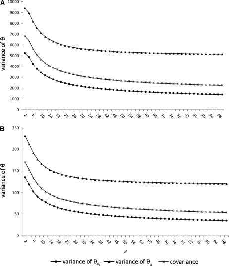
Figure 2 shows the relationship between d and the variance in the estimators for n = 100. When the ascertainment sample size is small compared to the size of the sample, the variances and covariances are greatly increased [for _d_ = 2 the variance of Tajima's θ ( ) is nearly doubled, and the variance of
  is nearly multiplied by four]. However, when d approaches n/2, the difference between the real variance and the estimated variance is drastically reduced.
Figure 2.—
The variance of Watterson's estimator of θ ( ) and Tajima's estimator of θ (
 ) and the covariance as a function of d calculated using estimated values of θ and θ2 for a sample of size n = 100. We performed 10,000 replicates. (A) θ = 150. (B) θ = 22.33.
Correction of Tajima's D:
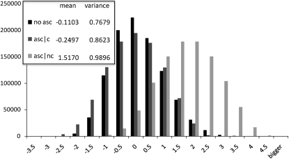
Figure 3 shows the distribution of Tajima's D and _D_C values for n = 50, d = 5, and θ = 150. When there is no ascertainment bias, the distribution of Tajima's D values using Equation 17 is identical to the one obtained using the standard method, with mean = −0.1103 in both cases, while when there is ascertainment bias and we do not apply the corrected formula, the distribution is greatly skewed toward positive values (mean = 1.5170). If the correction is applied to the simulated data suffering from the ascertainment bias, the nonascertained distribution is approximately recovered and its mean, −0.2497, gets closer to the nonascertainment one. However, because the correction is nonlinear, it does not match the original distribution exactly but is slightly skewed toward negative values compared to the original distribution and has a slightly larger variance. Neither the original Tajima's D in the absence of an ascertainment bias nor the current ascertainment corrected estimator in the presence of ascertainment bias has expectation equal to zero. Both rely on a ratio of two correlated statistics, so even though the numerator has expectation equal to zero, the expectation of the ratio is not equal to zero. Also, it is not surprising that the variance is slightly larger for the ascertainment corrected statistic. It suggests that some information has been lost by the ascertainment process. The same tendencies can be seen for the other values of θ explored (see supplemental data A).
Figure 3.—
The distribution of Tajima's D for data without ascertainment bias and without correction (no asc), for ascertained data with correction (asc | c), and for ascertained data without correction (asc | nc). The mean and the variance among estimates are shown in the inset. A value of θ = 150 was used, with n = 50, d = 5, and 1,000,000 replicates were performed.
Analysis of Perlegen data:
To illustrate the use of the correction of Tajima's D, we applied it to a Perlegen data set (Hinds et al. 2005), previously analyzed by Clark et al. (2005) without correcting for ascertainment bias. The Perlegen data were analyzed chromosome by chromosome, taking windows of 100 spanning 10 kb obtaining, on average, 12,221 windows per chromosome. A total of 74.47% of the windows have ≥10 SNPs and are, therefore, included for the comparison between the corrected and the uncorrected Tajima's D values.
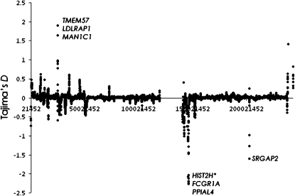
An example of the result, using windows of 500 kb on chromosome 1, is shown in Figure 4. Positive Tajima's D values (1.9) are found in the area containing the genes TMEM57, MAN1C1, and LDLRAP1. The former is a transmembrane protein and the second a mannosidase. The latter encodes for a cytosolic protein that interacts with the LDL receptor, and mutations in it have cause hypercholesterolemia, an autosomal recessive disorder (Mishra et al. 2005; Quagliarini et al. 2007). Negative Tajima's D values ∼ −2 were found in windows containing HIST2H*, FCGR1A, and PPIAL4, a histone cluster, a fragment of the IgG receptor, and the peptidylprolyl isomerase A, respectively. D values of −1.6 were found around the SRGAP2 gene, whose mRNA has been found in melanoma, germ cell tumors, chondrosarcoma, and retinoblastoma (Katoh and Katoh 2003).
Figure 4.—
The distribution of the ascertainment bias corrected Tajima's D on chromosome 1 in the human genome based on the Perlegen data. The genes with the most extreme D values are also indicated.
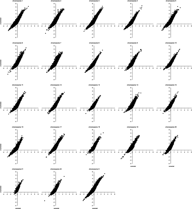
Figure 5 shows the correlation of Tajima's D results with and without correction for all chromosomes. As expected, the D values are higher than the _D_C values. We examine windows with extreme values of Tajima's D, which we have arbitrarily defined as those with values < −2 or >2, in more detail. While there are 210 windows with _D_C ≤ −2, there are only 17 windows with D ≤ −2. Likewise, there are 99 windows with _D_C ≥ 2 and 8317 with D ≥ 2. Table 1 summarizes the information about the 50 windows with the most extreme values of _D_C (25 lowest and 25 highest). Of the 25 windows with lowest values of _D_C, 3 would not be found among the 25 most significant windows using D, and 8, including the GPC3 gene, would be excluded on the basis of the D ≤ −2 criterion. Among the 25 most significant windows with positive values of _D_C, 10 of them are not included in the set of the 25 most extreme genes based on D. Among these windows there are genes such as BRCA1 or NF1. Fourteen of 15 genes are located on the X chromosome. A possible explanation is that selection on the X chromosome is more efficient because recessive mutations are exposed to selection in males (see, e.g., Schaffner 2004).
Figure 5.—
Correlation of Tajima's D results from Perlegen data with and without correction for all chromosomes.
TABLE 1.
Fifty windows with more extreme Tajima's D values for the corrected estimator
| Chromosome | Window | First SNP | Last SNP | Gene containing first SNP | Gene containing last SNP | Corrected Tajima's D | Uncorrected Tajima's D |
|---|---|---|---|---|---|---|---|
| 25 windows with lowest corrected Tajima's D | |||||||
| 19 | 1505 | rs11883009 | rs10775618 | — | AKAP8L | −3.282039 | −2.527051 |
| 22 | 1278 | rs16986494 | rs4035540 | TTC28 | CHEK2 | −3.200966 | −2.545256 |
| X | 1726 | rs16980685 | rs17320692 | — | — | −3.164725 | −2.499758 |
| X | 1722 | rs10521677 | rs17246666 | — | — | −3.110302 | −2.426383 |
| 19 | 1503 | rs16980448 | rs10775618 | BRD4 | AKAP8L | −3.049939 | −2.356206 |
| X | 2088 | rs16981582 | rs6528025 | CNKSR2 | CNKSR2 | −2.968399 | −2.151076 |
| 02 | 13306 | rs16849050 | rs16849021 | — | — | −2.958659 | −2.765536 |
| 03 | 1909 | rs10510486 | rs17005761 | KCNH8 | KCNH8 | −2.892485 | −2.138216 |
| X | 10073 | rs17331728 | rs17342441 | — | — | −2.867873 | −2.051048 |
| 16 | 1463 | rs17260976 | rs16966953 | PARN | NTAN1 | −2.856588 | −2.018186 |
| X | 13139 | rs17251454 | rs17000462 | GPC3 | GPC3 | −2.831727 | −1.991586 |
| 19 | 1497 | rs16980438 | rs4616406 | — | — | −2.813864 | −2.045236 |
| X | 13140 | rs7061117 | rs17000463 | GPC3 | GPC3 | −2.809700 | −1.991586 |
| 19 | 1171 | rs17001730 | rs10424893 | ZNF700 | — | −2.802120 | −1.927546 |
| 06 | 6799 | rs17446192 | rs4710655 | — | — | −2.795281 | −2.372185 |
| X | 10074 | rs16984144 | rs10521499 | BHLHB9 | — | −2.794317 | −2.070374 |
| 17 | 6325 | rs16961696 | rs2221741 | — | — | −2.761039 | −2.083343 |
| X | 1720 | rs12845504 | rs17246666 | — | — | −2.754714 | −2.094886 |
| 19 | 1499 | rs16980438 | rs16980462 | — | — | −2.706380 | −2.012035 |
| 07 | 7214 | Not found | rs2353082 | Not found | BAZ1B | −2.663340 | −1.858293 |
| 17 | 6324 | rs16961697 | rs2221741 | — | — | −2.661940 | −2.045867 |
| 01 | 5148 | rs12094202 | rs10489546 | OSBPL9 | OSBPL9 | −2.659012 | −1.964506 |
| 19 | 1501 | rs8104223 | rs10775618 | BRD4 | AKAP8L | −2.654787 | −1.953696 |
| 08 | 9984 | rs16897122 | rs2029596 | — | VPS13B | −2.652911 | −1.812917 |
| 06 | 10935 | rs17070142 | rs351730 | SESN1 | — | −2.645325 | −1.770006 |
| 25 windows with highest corrected Tajima's D | |||||||
| 01 | 11083 | rs1774778 | rs17026872 | — | — | 3.131594 | 5.174721 |
| X | 13405 | rs5975710 | rs6633822 | MAP7D3 | GPR112 | 3.069725 | 5.475525 |
| 01 | 11084 | rs1774778 | rs325910 | — | — | 2.749263 | 4.683911 |
| X | 13061 | rs5975352 | rs17324216 | HS6ST2 | HS6ST2 | 2.743219 | 4.817528 |
| 04 | 13648 | rs7658327 | rs13143611 | — | — | 2.723831 | 5.389725 |
| 05 | 7065 | rs986217 | rs1017225 | — | BDP1 | 2.717593 | 4.800969 |
| X | 12501 | rs203491 | rs5931921 | — | — | 2.682832 | 4.922305 |
| 18 | 3626 | rs2217945 | rs7232770 | — | — | 2.656100 | 5.096458 |
| 04 | 12950 | rs1870687 | rs12510308 | LARP2 | — | 2.645268 | 4.870015 |
| 10 | 12713 | rs10794030 | rs7918092 | DHX32 | FANK1 | 2.590828 | 4.981469 |
| 09 | 8180 | rs7044691 | rs9410888 | GKAP1 | KIF27 | 2.577577 | 4.565764 |
| 01 | 11082 | rs1342353 | rs17026872 | — | — | 2.553143 | 4.457859 |
| X | 13109 | rs5975387 | rs5977860 | — | GPC4 | 2.551131 | 4.648231 |
| 03 | 4834 | rs725310 | rs734071 | FBXW12 | SCOTIN | 2.534127 | 4.769015 |
| 04 | 5577 | rs10434442 | rs17085274 | KDR | KDR | 2.531075 | 4.478948 |
| X | 13062 | rs17317147 | rs5933229 | HS6ST2 | HS6ST2 | 2.523093 | 4.457818 |
| 09 | 8024 | rs2788113 | rs12686026 | — | — | 2.511495 | 4.827204 |
| 12 | 5603 | rs537482 | rs511752 | — | ARHGAP9 | 2.509088 | 4.637981 |
| 17 | 2954 | rs12948444 | rs2952991 | NF1 | NF1 | 2.501910 | 4.508276 |
| 03 | 9662 | rs6806361 | rs1533148 | — | — | 2.484018 | 4.814285 |
| 17 | 4158 | rs3950989 | rs8070085 | BRCA1 | NBR1 | 2.479324 | 4.643384 |
| X | 13110 | rs5975387 | rs17317322 | — | GPC4 | 2.457019 | 4.491652 |
| 06 | 7949 | rs9352669 | rs956550 | IRAK1BP1 | — | 2.455673 | 5.427745 |
| 14 | 4683 | rs9323475 | rs17182817 | GPHN | GPHN | 2.444739 | 4.476493 |
| 03 | 9663 | rs6806361 | rs9833997 | — | — | 2.428898 | 4.650462 |
DISCUSSION
We have here derived estimators of the population genetic parameter θ, and the variances and covariances of the estimators, under a model with ascertainment bias. This leads us to an ascertainment correction of Tajima's D. We note that similar corrections could easily be derived for other statistics as well, particularly if they can be written as functions of site frequency spectrum, i.e., η i, i = 1, 2, … , n − 1. Statistics such as Fu and Li's D (Fu and Li 1993) and Fay and Wu's H (Fay and Wu 2000) are included in this category. We also emphasize that while the ascertainment scheme here is quite specific, and the results may therefore not always apply to real data, all results are expressed in terms of the probability of ascertainment of a SNP as a function of its frequency,  . It is, therefore, quite trivial to extend this work to other ascertainment schemes, including the ones considered in Nielsen et al. (2005), as long as appropriate ascertainment information is available.
The methods applied here assume that there is no intralocus recombination, as expressions explicitly incorporating recombination are not tractable for Tajima's D. There is a tradition for applying Tajima's D and other similar statistics that are derived assuming no recombination, even in the presence of recombination. As recombination tends to reduce the variance of Tajima's D among regions, such applications are considered conservative (e.g., Ramírez-Soriano et al. 2008).
The analysis of the Perlegen data illustrates that ascertainment bias correction is of great importance when analyzing SNP genotyping data. Even when just applying outlier approaches in studies of natural selection, the ranking of different genes is likely to change with and without ascertainment bias correction. Likewise, any study aimed at quantifying variability on the basis of typical SNP data will be challenged by the ascertainment bias. It is, therefore, highly desirable that SNP genotyping projects keep close track of the SNP discovery/selection protocols used. Only when such detailed data regarding these protocols are available will it be possible to make accurate ascertainment bias corrections of the data.
A computer program implementing the ascertainment bias corrections discussed in this article can be downloaded from http://www.snpator.com/public/downloads/aRamirez/tajimasDCorrector/. A list of corrected Tajima's D values for different regions of the human genome can be found in supplemental data B.
Acknowledgments
We thank Marta Melé and Francesc Calafell for their comments on this manuscript. This work was supported by National Institutes of Health grant U01HL084706 and by the Danish National Science Council.
References
- Altshuler, D., V. J. Pollara, C. R. Cowles, W. J. Van Etten, J. Baldwin et al., 2000. An SNP map of the human genome generated by reduced representation shotgun sequencing. Nature 407 513–516. [DOI] [PubMed] [Google Scholar]
- Bamshad, M., and S. P. Wooding, 2003. Signatures of natural selection in the human genome. Nat. Rev. Genet. 4 99–111. [DOI] [PubMed] [Google Scholar]
- Carlson, C. S., M. A. Eberle, L. Kruglyak and D. A. Nickerson, 2004. Mapping complex disease loci in whole-genome association studies. Nature 429 446–452. [DOI] [PubMed] [Google Scholar]
- Carlson, C. S., J. D. Smith, I. B. Stanaway, M. J. Rieder and D. A. Nickerson, 2006. Direct detection of null alleles in SNP genotyping data. Hum. Mol. Genet. 15 1931–1937. [DOI] [PubMed] [Google Scholar]
- Clark, A. G., M. J. Hubisz, C. D. Bustamante, S. H. Williamson and R. Nielsen, 2005. Ascertainment bias in studies of human genome-wide polymorphism. Genome Res. 15 1496–1502. [DOI] [PMC free article] [PubMed] [Google Scholar]
- Crawford, D. C., D. T. Akey and D. A. Nickerson, 2005. The patterns of natural variation in human genes. Annu. Rev. Genomics Hum. Genet. 6 287–312. [DOI] [PubMed] [Google Scholar]
- Durrett, R., 2008. Probability Models for DNA Sequence Evolution (Probability and Its Applications). Springer, Berlin/Heidelberg, Germany/New York.
- Fay, J. C., and C. I. Wu, 2000. Hitchhiking under positive Darwinian selection. Genetics 155 1405–1413. [DOI] [PMC free article] [PubMed] [Google Scholar]
- Fu, Y. X., 1995. Statistical properties of segregating sites. Theor. Popul. Biol. 48 172–197. [DOI] [PubMed] [Google Scholar]
- Fu, Y. X., and W. H. Li, 1993. Statistical tests of neutrality of mutations. Genetics 133 693–709. [DOI] [PMC free article] [PubMed] [Google Scholar]
- Hinds, D. A., L. L. Stuve, G. B. Nilsen, E. Halperin, E. Eskin et al., 2005. Whole-genome patterns of common DNA variation in three human populations. Science 307 1072–1079. [DOI] [PubMed] [Google Scholar]
- Hudson, R. R., 2002. Generating samples under a Wright-Fisher neutral model of genetic variation. Bioinformatics 18 337–338. [DOI] [PubMed] [Google Scholar]
- International HapMap Consortium, 2007. A second generation human haplotype map of over 3.1 million SNPs. Nature 449 851–861. [DOI] [PMC free article] [PubMed] [Google Scholar]
- Katoh, M., and M. Katoh, 2003. FNBP2 gene on human chromosome 1q32.1 encodes ARHGAP family protein with FCH, FBH, RhoGAP and SH3 domains. Int. J. Mol. Med. 11 791–797. [PubMed] [Google Scholar]
- Kreitman, M., and A. Di Rienzo, 2004. Balancing claims for balancing selection. Trends Genet. 20 300–304. [DOI] [PubMed] [Google Scholar]
- Marth, G. T., E. Czabarka, J. Murvai and S. T. Sherry, 2004. The allele frequency spectrum in genomewide human variation data reveals signals of differential demographic history in three large world populations. Genetics 166 351–372. [DOI] [PMC free article] [PubMed] [Google Scholar]
- Mead, S., M. P. Stumpf, J. Whitfield, J. A. Beck, M. Poulter et al., 2003. Balancing selection at the prion protein gene consistent with prehistoric kurulike epidemics. Science 300 640–643. [DOI] [PubMed] [Google Scholar]
- Mishra, S. K., P. A. Keyel, M. A. Edeling, A. L. Dupin, D. J. Owen et al., 2005. Functional dissection of an AP-2 beta2 appendage-binding sequence within the autosomal recessive hypercholesterolemia protein. J. Biol. Chem. 280 19270–19280. [DOI] [PubMed] [Google Scholar]
- Nielsen, R., 2000. Estimation of population parameters and recombination rates from single nucleotide polymorphisms. Genetics 154 931–942. [DOI] [PMC free article] [PubMed] [Google Scholar]
- Nielsen, R., 2004. Population genetic analysis of ascertained SNP data. Hum. Genomics 1 218–224. [DOI] [PMC free article] [PubMed] [Google Scholar]
- Nielsen, R., and J. Signorovitch, 2003. Correcting for ascertainment biases when analyzing SNP data: applications to the estimation of linkage disequilibrium. Theor. Popul. Biol. 63 245–255. [DOI] [PubMed] [Google Scholar]
- Nielsen, R., M. J. Hubisz and A. G. Clark, 2004. Reconstituting the frequency spectrum of ascertained single-nucleotide polymorphism data. Genetics 168 2373–2382. [DOI] [PMC free article] [PubMed] [Google Scholar]
- Nielsen, R., S. Williamson, Y. Kim, M. J. Hubisz, A. G. Clark et al., 2005. Genomic scans for selective sweeps using SNP data. Genome Res. 15 1566–1575. [DOI] [PMC free article] [PubMed] [Google Scholar]
- Picoult-Newberg, L., T. E. Ideker, M. G. Pohl, S. L. Taylor, M. A. Donaldson et al., 1999. Mining SNPs from EST databases. Genome Res. 9 167–174. [PMC free article] [PubMed] [Google Scholar]
- Polanski, A., and M. Kimmel, 2003. New explicit expressions for relative frequencies of single-nucleotide polymorphisms with application to statistical inference on population growth. Genetics 165 427–436. [DOI] [PMC free article] [PubMed] [Google Scholar]
- Ramírez-Soriano, A., S. E. Ramos-Onsins, J. Rozas, F. Calafell and A. Navarro, 2008. Statistical power analysis of neutrality tests under demographic expansions, contractions and bottlenecks with recombination. Genetics 179 555–567. [DOI] [PMC free article] [PubMed] [Google Scholar]
- Quagliarini, F., J. C. Vallve, F. Campagna, A. Alvaro, F. J. Fuentes-Jimenez et al., 2007. Autosomal recessive hypercholesterolemia in Spanish kindred due to a large deletion in the ARH gene. Mol. Genet. Metab. 92 243–248. [DOI] [PubMed] [Google Scholar]
- Ramos-Onsins, S. E., and J. Rozas, 2002. Statistical properties of new neutrality tests against population growth. Mol. Biol. Evol. 19 2092–2100. [DOI] [PubMed] [Google Scholar]
- Sabeti, P. C., D. E. Reich, J. M. Higgins, H. Z. Levine, D. J. Richter et al., 2002. Detecting recent positive selection in the human genome from haplotype structure. Nature 419 832–837. [DOI] [PubMed] [Google Scholar]
- Sabeti, P. C., S. F. Schaffner, B. Fry, J. Lohmueller, P. Varilly et al., 2006. Positive natural selection in the human lineage. Science 312 1614–1620. [DOI] [PubMed] [Google Scholar]
- Schaffner, S. F., 2004. The X chromosome in population genetics. Nat. Rev. Genet. 5 43–51. [DOI] [PubMed] [Google Scholar]
- Soldevila, M., F. Calafell, A. Helgason, K. Stefansson and J. Bertranpetit, 2005. Assessing the signatures of selection in PRNP from polymorphism data: results support Kreitman and di Rienzo's opinion. Trends Genet. 21 389–391. [DOI] [PubMed] [Google Scholar]
- Tajima, F., 1989. Statistical method for testing the neutral mutation hypothesis by DNA polymorphism. Genetics 123 585–595. [DOI] [PMC free article] [PubMed] [Google Scholar]
- Tang, K., K. R. Thornton and M. Stoneking, 2007. A new approach for using genome scans to detect recent positive selection in the human genome. PLoS Biol. 5 e171. [DOI] [PMC free article] [PubMed] [Google Scholar]
- Voight, B. F., S. Kudaravalli, X. Wen and J. K. Pritchard, 2006. A map of recent positive selection in the human genome. PLoS Biol. 4 e72. [DOI] [PMC free article] [PubMed] [Google Scholar]
- Wakeley, J., R. Nielsen, S. N. Liu-Cordero and K. Ardlie, 2001. The discovery of single-nucleotide polymorphisms–and inferences about human demographic history. Am. J. Hum. Genet. 69 1332–1347. [DOI] [PMC free article] [PubMed] [Google Scholar]
- Wang, Y., L. P. Zhao and S. Dudoit, 2006. A fine-scale linkage-disequilibrium measure based on length of haplotype sharing. Am. J. Hum. Genet. 78 615–628. [DOI] [PMC free article] [PubMed] [Google Scholar]
- Watterson, G. A., 1975. On the number of segregating sites in genetical models without recombination. Theor. Popul. Biol. 7 256–276. [DOI] [PubMed] [Google Scholar]
- Williamson, S. H., M. J. Hubisz, A. G. Clark, B. A. Payseur, C. D. Bustamante et al., 2007. Localizing recent adaptive evolution in the human genome. PLoS Genet. 3 e90. [DOI] [PMC free article] [PubMed] [Google Scholar]
- Wooding, S., 2004. Natural selection: sign, sign, everywhere a sign. Curr. Biol. 14 R700–R701. [DOI] [PubMed] [Google Scholar]
