Multivariate Cutoff Level Analysis (MultiCoLA) of large community data sets (original) (raw)
Abstract
High-throughput sequencing techniques are becoming attractive to molecular biologists and ecologists as they provide a time- and cost-effective way to explore diversity patterns in environmental samples at an unprecedented resolution. An issue common to many studies is the definition of what fractions of a data set should be considered as rare or dominant. Yet this question has neither been satisfactorily addressed, nor is the impact of such definition on data set structure and interpretation been fully evaluated. Here we propose a strategy, MultiCoLA (Multivariate Cutoff Level Analysis), to systematically assess the impact of various abundance or rarity cutoff levels on the resulting data set structure and on the consistency of the further ecological interpretation. We applied MultiCoLA to a 454 massively parallel tag sequencing data set of V6 ribosomal sequences from marine microbes in temperate coastal sands. Consistent ecological patterns were maintained after removing up to 35–40% rare sequences and similar patterns of beta diversity were observed after denoising the data set by using a preclustering algorithm of 454 flowgrams. This example validates the importance of exploring the impact of the definition of rarity in large community data sets. Future applications can be foreseen for data sets from different types of habitats, e.g. other marine environments, soil and human microbiota.
INTRODUCTION
Community ecologists traditionally deal with data sets consisting of large tables of samples by ‘species’ (hereafter referred to as ‘types’). The scientific community has yet not reached a general agreement on the optimal way to deal with rare types (1): for some, rare types are noise in data sets which may originate from sampling artifacts and thus do not represent the whole community. Rare types are often removed so as to decrease the large amount of zeros stored in data sets, and to reduce the challenging task of their taxonomic identification (1). For others, rare types are valuable as they may provide critical insights into the functioning of ecosystems such as resistance against invasive species or into the likely existence of multiple niches (1). It is thus left at the discretion of the authors to define their own concept of rarity: rare plants and animals may be defined according to their restricted geographical distribution (2) or to their low proportions in data sets (3).
In microbial ecology, the current revolution in high-throughput DNA sequencing technology has revealed the existence of a ‘rare biosphere’, consisting of the many microbial types displaying long distribution tails in rank-abundance curves (4,5). Because sequencing artifacts may produce chimeric types (6), several studies have put into doubt the true existence of rare types in the high-throughput sequencing data sets and have provided various ways to trim and correct sequences: for instance, clustering threshold at 97% sequence identity (7) on 454 massively parallel tag sequencing (MPTS) data or a flowgram-based preclustering algorithm (8) may be applied. When rare types are not considered as artifacts, they can be defined by applying arbitrary abundance cutoffs to the original data set (9). However, the effects of the definition of rare organisms on the stability of the data structure and ecological conclusions that derive from the resulting, truncated data sets have not been examined so far.
We propose a new approach, Multivariate Cutoff Level Analysis (MultiCoLA), to systematically explore how large community data sets are affected by different definitions of rarity. First, MultiCoLA truncates the original data set by discarding rare types according to successive increasing abundance cutoffs. The effects of removing rare types are then measured at the levels of (i) variation of data set structure, (ii) amounts of extracted variation between the original and the truncated data sets and (iii) the ecological interpretation of the original and each truncated data sets when environmental parameters are available.
MATERIALS AND METHODS
Data set
In this study, the analyses were performed on a data set consisting of hyper-variable V6 sequences of the 16S rRNA gene, which were obtained from the application of 454 MPTS on temperate subtidal sandy samples at three sediment depth layers (0–15 cm depth, with a 5-cm interval) taken over 2 years (2005–2006). Detailed sample processing and DNA extraction has been described earlier (10) and the 454 MPTS of the extracted DNA was processed as described previously (5). The output from 454 MPTS was retrieved from the publicly available Visualization and Analysis of Microbial Populations Structure (VAMPS) web site (http://vamps.mbl.edu/). An automatic annotation pipeline [Global Alignment for Sequence Taxonomy (GAST) (5)] using several known databases (Entrez Genome, RDP and SILVA) allowed the taxonomic assignment of the sequences. Despite the limitations of current databases, only 6% of sequences from this data set were not taxonomically identified at all. However, about 20% of sequences were annotated from the phylum to the genus level. In this study, the analyses were performed by defining OTUs (operational taxonomic units) as unique sequences (i.e. sequences differing by at least one base were considered as different OTUs. Note, however, that MultiCoLA could also have been applied to sequence subsets based on another OTU definition) and the following subsets were considered: (i) all, unannotated sequences that we referred to as ‘OTU whole data set (DS)’, (ii) on the 20% fully annotated sequences (i.e. from phylum to genus levels and the corresponding OTU level) and (iii) on PyroNoise-corrected data defined at different percentages of sequence similarity.
Data analyses
Truncated tables
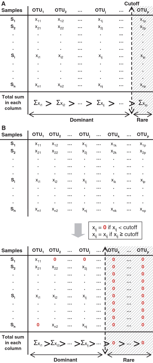
Data sets were analyzed by applying two types of cutoff abundance levels (Figure 1): (i) Whole-data set-based cutoffs_:_ truncated matrices were obtained by removing chosen proportions (0, 1, 5–95 and 99%) of rare OTUs from the total sum of sequences in the data set (Figure 1A). The original data set was first sorted according to the decreasing number of sequences per OTU. Then low-abundance OTUs were removed according to the given cutoff levels. (ii) Sample-based cutoffs: a total of 15 cutoffs were selected from 1 to 208 total number of sequences per OTU per sample (because certain samples did not contain any more OTUs for cutoff levels higher than 208 sequences, i.e. 208 was the lowest number of the maximum OTU occurrences per sample), in order to select OTUs with more sequences than the applied cutoff (Figure 1B). This number is obviously specific to each data set and should be taken into consideration if one wants to consider the same number of samples in all comparative analyses.
Figure 1.
Two ways of assigning rarity cutoffs to the original data set. (A) In the data set-based approach, cutoff levels are assigned to the original data set according to several percentages (0, 1, 5–95 and 99%) of the total number of sequences in the data set. The data set was sorted according to the decreasing total sum of OTU sequences (columns, here) before selecting out rare OTUs. For instance, a cutoff assignment of 1% removes 1% of the low-abundant OTUs. (B) In the sample-based approach, cutoff levels are assigned to the original data set according to the occurrence (1–208 sequences) of each OTU in each sample. The maximum cutoff (here, 208) was chosen according to the lowest number of the maximum OTU occurrences in all samples; this is the limit when some samples did not contain any more OTUs. For example, the assignment of a cutoff level of 3 removes OTUs occurring less than three times in each sample.
Analyses of changes in bacterial community structure and in main patterns of community variation
Pairwise distance matrices were calculated from the data (original and truncated matrices) using the Bray–Curtis dissimilarity index (11). The resulting dissimilarity matrices were compared with one another using the non-parametric Spearman rho correlation coefficient (12), which ranges from 0 to 1 (a score closer to 1 indicates higher correlations between dissimilarity matrices).
Variations in the main axes of extracted variation in community structure were explored via non-metric multidimensional scaling [NMDS (13)], a method commonly used to identify diversity patterns from molecular fingerprinting results (14). The Procrustes method (15) was then used to compare the NMDS ordination results from the original distance matrix with those from the truncated distance matrices. Procrustes rotation produces an R value that ranges from 0 to 1 [a score closer to 1 indicates highest similarities between the NMDS results (16)]. In other words, this approach enables to quantify the agreement between the most important axes of extracted variation from the original versus truncated data sets. This is particularly relevant because multivariate analyses that are typically applied to such data sets generally focus on the first few axes of main biological variation in the data.
In both profiles of data structure and extracted variation, a limitation is that one cannot calculate either the confidence interval or the significance of each pairwise comparison (i.e. for each single point). This is because the truncated matrices depend on the original matrix and testing correlations would only make sense in the case of data set independence (17,18). Yet, those limitations are not critical to our approach because we are more interested in overall changes in profiles rather than single-point variation or estimation. Indeed, the emphasis here is to measure (such as an index would do) the deviation from the signals in the original data set under the various hypothetical scenarios, i.e. when applying various cutoff levels.
Relationships between community structure and environment
For illustration purposes, four major contextual parameters [silicate, phosphate, ammonium and cell abundance from Böer _et al._ (10), which were log10-transformed prior to analyses] were used to investigate the relationships between the bacterial community structure (at successive assigned cutoffs and taxonomic levels) and environmental parameters. Each response community data set was Hellinger-transformed as recommended when dealing with data sets to be analyzed via linear multivariate models (19). Canonical variation partitioning (19,20) was then applied to the community data to test for the effects of each environmental variable (silicate, phosphate, ammonium and cell abundance) and their covariation on microbial community structure (21). Significances of the global and partial regression models were determined by using 1000 data permutations.
Creation of the MultiCoLA scripts
All statistical analyses were carried out using the R statistical environment (22), and specific routines in the vegan (23) and MASS (24) packages. The resulting MultiCoLA scripts are available at http://www.ecology-research.com. Some MultiCoLA scripts require some time and a certain computing power (10 min of calculations for an example matrix with 1000 OTUs on an Intel Pentium 4), but this may vary as a function of data set size and complexity, and choice of the analyses (i.e. Spearman correlations, Procrustes correlation or variation partitioning at multiple cutoff levels).
RESULTS AND DISCUSSION
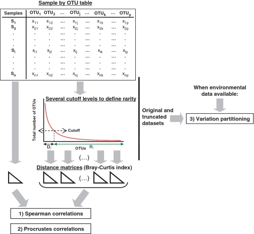
Two approaches may be applied to truncate the original data set when removing an increasing proportion of rare types: either the whole data set is considered or each sample is considered individually (Figure 1). Because there is no reason to a priori choose a given threshold value, various cutoffs need to be systematically applied to explore their effects. The resulting, truncated data sets are then evaluated at three levels: first, the data sets are converted to sample-by-sample dissimilarity matrices (e.g. here we used the Bray–Curtis coefficient to calculate the dissimilarity between samples but other dissimilarity coefficients may be used) and those matrices are compared with the matrix produced by the whole dataset using non-parametric Spearman correlations (Figure 2), so as to assess changes in data structure. Second, the amounts of extracted ecological variation, obtained by the application of the NMDS ordination, in the truncated and original data sets are compared by Procrustes rotation (i.e. a measure of the correlation between two ordination solutions). Third, when contextual parameters (e.g. space, time or environment) are available, it is possible to systematically compare the ecological interpretation of each truncated data set with that of the original data set. This is achieved by partitioning the biological variation from the different truncated data sets as a function of explanatory variables (Materials and Methods section).
Figure 2.
MultiCoLA steps. After truncating the original table according to various abundance cutoff levels, the effects of specific rarity definitions are tested by applying three types of analyses: (1) Variations in data set structure are established based on non-parametric correlations of pairwise distance matrices (e.g. calculated with the Bray–Curtis coefficient). (2) The amounts of extracted community variation (using NMDS) from the original data and the truncated data sets are compared by Procrustes correlations. (3) When additional parameters are available, the biological variation that can be explained by environmental parameters in the original and in the truncated data sets are then systematically compared. D, dominant OTUs; R, rare OTUs.
We applied MultiCoLA to a large 454 MPTS data set representing a case of high microbial diversity retrieved from temperate coastal sediments (10), which included a considerable amount of singletons (68% unique OTUs with a single sequence and 10% unique sequences in the whole data set) and low-abundant types. Another level of interest came from the fact that many sequences could also be taxonomically classified by applying the GAST taxonomic pipeline (5). It was thus possible to systematically explore the effects of rarity definition on the structure and interpretation of a data set at different taxonomic levels.
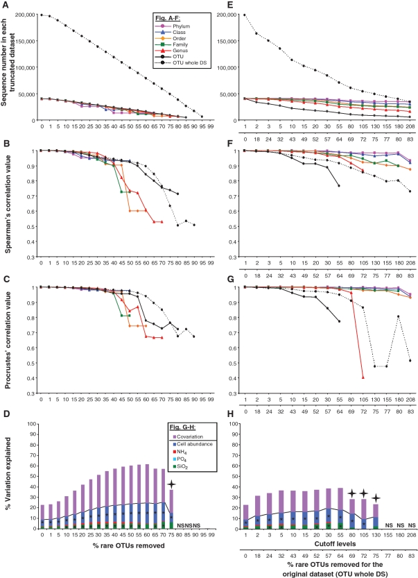
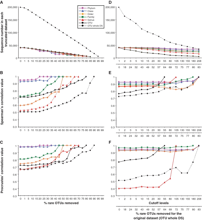
The systematic truncation of the whole data set produced a quasi linear decrease in sequence number as a function of increasing cutoff levels, and a similar trend was observed for the taxonomically annotated OTUs (Figure 3A). When the structure of community tables were compared between the truncated and the original matrices (Figure 3B), little variation in data structure was observed up to a removal threshold of 40% of the rare parts of the data set, indicating robustness in the signal far beyond the usual removal of singletons. Beyond the 40% threshold, the correlation coefficients greatly varied in a non-linear and non-predictive fashion, with higher taxonomic levels mostly associated with higher correlation values. When the most important patterns of extracted variation were compared between the various truncated and the original data sets (Figure 3C), a similar picture emerged with 40% representing a cutoff level up to which very little change in extracted variation could be observed. Beyond this threshold, Procrustes coefficients also greatly varied in a non-predictable and non-linear way, again regardless of the taxonomic level of the analysis.
Figure 3.
MultiCoLA profiles for data set structure, most important axes of extracted variation and interpretation of biological variation based on the data set-based (A–D) and sample-based (E–H) approaches. (A, E) Abundance of dominant OTUs in each truncated data set at the phylum, class, order, family, genus and OTU levels. A black solid line indicates comparisons at the OTU level for the data set with a complete annotation and a black dashed line indicates the OTU level with the whole data set (OTU whole DS). (B, F) Non-parametric Spearman correlations comparing the deviation in complete data structure between the original matrix and truncated matrices. (C, G) Comparison of most important axes of extracted variation between the original and truncated data sets. (D, H) Partitioning of the biological variation at the OTU level (all OTUs) into the respective effects of environmental factors (nutrients and cell abundance). Negative values, unexplained variation and non-significant models are not shown. SiO2, silicate; PO4, phosphate; NH4, ammonium; covariation of any of the four environmental factors is represented under the same category. Asterisk indicates a significant effect of the pure factors (P < 5%), whereas ‘NS’ indicates non-significant models. A cross indicates non-significant Bonferroni corrected models. Lacking points or bars are due to sample loss by applying a given cutoff to the original data set. In (E–H), the upper _x_-axis corresponds to cutoff levels defined as a function of the sample-based approach, and the lower _x_-axis represents the corresponding proportion of removed sequences in the OTU data set (all OTUs). This enables the comparison of the data set-based approach with the sample-based approach. Note that (D and H) have a different legend than (A–C) and (E–G).
When the truncated data sets were further analyzed as a function of environmental parameters, a surprising picture emerged (Figure 3D): nutrients (phosphate, silicate and ammonium) and total cell abundance seemed to consistently affect community variation at different cutoff levels. Not surprisingly, more explained variation was obtained overall when data complexity was reduced via the application of increasing cutoff levels or at higher taxonomic levels (Supplementary Figure S1). Noticeably, different multivariate models could be retained at each cutoff level or at each taxonomic level of the analyses, indicating that each truncated data set may be explained by slightly different combinations or covariations of environmental factors (Supplementary Tables S1–S7). It seemed overall that the rather broad taxonomic classification of the sequences was sufficient to describe general ecological patterns and that the interpretation of the effects of the structuring factors was robust and would not be affected by the removal of a large fraction of the rare types.
When applying the sample-based approach to the data to reveal changes in data structure and extracted variation (Figure 3F and G, respectively), changes in data structure varied in a narrower range (Spearman correlation coefficient from 0.8 to 1), while changes in extracted ecological variation varied over a larger range (Procrustes correlations from 0.5 to 1) and less predictably, as compared with their counterparts from the whole-data set approach (Figure 3B and C, respectively). A similar critical threshold of 35–40% for which profiles became more dissimilar from each other was also observed. For instance, by removing sequences occurring less than five times in the data set (i.e. removing 32% of all sequences), only a small drop in Spearman correlation coefficient to 0.98 would be observed, as compared with the original data set matrix, regardless of the taxonomic affiliation of the sequences (Figure 3F). Yet, the explained variations in community structure as explained by nutrients and cell abundance (Figure 3D and H) were qualitatively similar to those based on the data set approach. More variation was again explained at higher taxonomic levels (Supplementary Figure S2 and Tables S8–S14). Therefore, choosing the sample- or data set- based approach would lead to the same ecological conclusions, despite their contrasting effects on data structure and amount of extracted ecological variation.
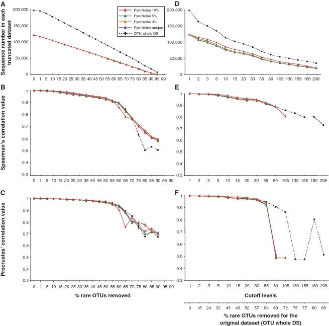
Because sequencing and PCR noise may generate spurious, low-abundance types, especially in high-throughput sequencing data sets (6), two strategies have been proposed to correct for sequence artifacts: a clustering threshold at 97% sequence identity (7) or a flowgram-based preclustering algorithm (8). A central question is therefore whether the afore-described variation observed in MultiCoLA profiles could be due to the presence of sequence artifacts. When MultiCoLA was applied to PyroNoise-corrected data (Supplementary Table S15), both the data set-based (Figure 4A–C) and sample-based (Figure 4D–F) approaches produced very similar profiles as those obtained with uncorrected data. The main differences consisted of generally less fluctuations in the profiles and of higher cutoff levels of 55–60% (i.e. 30–55 individual sequence abundance in the data set) that should be reached to drastically deviate from the signal in the original data set. Explanation of the community variation by additional environmental parameters yielded the same conclusions as with uncorrected data (Supplementary Figure S3). Therefore, we can conclude that the observed variations in profiles at different cutoff and taxonomic levels were mostly due to non-technical fluctuations in the data, i.e. to real structural and ecological characteristics of the studied data sets.
Figure 4.
MultiCoLA profiles for data set structure and most important axes of extracted variation based on the data set (A–C) and sample (D–F) cutoff approaches for PyroNoise-corrected 454 MPTS data and the original 454 MPTS data set at the OTU level. Different colored lines indicate PyroNoise-corrected data sets whose sequences were further clustered at various sequence dissimilarity values. See Figure 3 for further details.
In this study, the original data set was used as reference for the MultiCoLA profiles, because usually one wants to remove only a small fraction of the data. Yet, it is also possible to choose the table of the most abundant types as reference for comparisons, so as to assess the effects of an increasing amount of rare types in the data set. By doing so (Figure 5), different profiles and fluctuation patterns could be observed, indicating a significant impact of the addition of rare types on data structure and ecological interpretation. Another possibility of analysis is to systematically remove the abundant fraction from each truncated data set and thus only retain the rare types (Supplementary Figure S4). This approach mimics the addition of an increasing amount of dominant types in the data set, and would enable a characterization of the data structure and ecological patterns, or lack of, present within the rare fraction of any data set. The resulting profiles and patterns (Supplementary Figure S4) were different from those obtained by systematically keeping the dominant fractions (Figure 3), suggesting that the rare fraction has a different structure and ecological signal than the more dominant fraction of the community. This observation opens the door to many new questions, but their exploration would go beyond the scope of the current study. In any case, these observations exemplify the usefulness of MultiCoLA to generate new knowledge about the nature of rarity in data sets.
Figure 5.
MultiCoLA profiles using the matrix with the most abundant OTUs as a reference for the comparison with the truncated matrices. (A–C) are based on the data set-based approach and (D–F) on the sample-based approach. See Figure 3 for further descriptions of each panel.
In conclusion, MultiCoLA enables a systematic and data-driven exploration of the impact of rarity or dominance of specific fractions of large community data sets and on their further ecological interpretations. This would be especially useful for data sets containing a large fraction of singletons, as found in previous high-throughput Sanger sequencing data sets [e.g. from clone libraries (25) or shotgun sequencing libraries (26)], and in ongoing, high-throughput 16S rRNA-based pyrosequencing projects [e.g. the International Census of Marine Microbes (ICoMM) (5,9), http://icomm.mbl.edu], and high-throughput metagenomic projects [e.g. the International Soil Metagenome Sequencing Consortium (Terragenome) (27), http://www.terragenome.org/; or the International Human Microbiome Consortium (IHMC) (28), http://www.human-microbiome.org/] where the rare sequence issue is generally addressed arbitrarily [e.g. a threshold of two reads was chosen to identify a gene in a human microbiome metagenomic data set (28)]. This analytical approach will also help scientists to move beyond the debate of sequence accuracy and in the future, it would be particularly interesting to determine how the threshold range of profile stability varies as a function of sequencing strategy, data set sizes, samples or habitat types.
The MultiCoLA software with its respective manual and examples are available at: http://www.ecology-research.com.
SUPPLEMENTARY DATA
Supplementary Data are available at NAR Online.
FUNDING
This work was supported by the Marie Curie Early Stage Training fellowship Site in Marine Microbiology (MarMic EST contract MEST-CT-2004-007776 to A.G.); the International Max Planck Research School of Marine Microbiology (to A.G.); the Max Planck Society (to A.R.). The sequencing was financed by a W.M. Keck Foundation award to the Marine Biological Laboratory at Woods Hole, MA. This is a contribution to the International Census of Marine Microbes (ICoMM). Funding for open access charge: Max Planck Society.
Conflict of interest statement. None declared.
Supplementary Material
[Supplementary Data]
ACKNOWLEDGEMENTS
We acknowledge Antje Boetius for helpful suggestions and discussions, Susan M. Huse and Philip R. Neal for curating and annotating the pyrotag sequences; Pierre Legendre for helpful statistical discussions.
REFERENCES
- 1.Gauch HG. Multivariate Analyses in Community Ecology. Cambridge: Cambridge University Press; 1982. [Google Scholar]
- 2.Prendergast JR, Quinn RM, Lawton JH, Eversham BC, Gibbons DW. Rare species, the coincidence of diversity hotspots and conservation strategies. Nature. 1993;365:335–337. [Google Scholar]
- 3.Magurran AE, Henderson PA. Explaining the excess of rare species in natural species abundance distributions. Nature. 2003;422:714–716. doi: 10.1038/nature01547. [DOI] [PubMed] [Google Scholar]
- 4.Pedrós-Alió C. Marine microbial diversity: can it be determined? Trends Microbiol. 2006;14:257–263. doi: 10.1016/j.tim.2006.04.007. [DOI] [PubMed] [Google Scholar]
- 5.Sogin ML, Morrison HG, Huber JA, Welch DM, Huse SM, Neal PR, Arrieta JM, Herndl GJ. Microbial diversity in the deep sea and the underexplored “rare biosphere”. Proc. Natl Acad. Sci. USA. 2006;103:12115–12120. doi: 10.1073/pnas.0605127103. [DOI] [PMC free article] [PubMed] [Google Scholar]
- 6.Quinlan AR, Stewart DA, Stromberg MP, Marth GT. Pyrobayes: an improved base caller for SNP discovery in pyrosequences. Nat. Methods. 2008;5:179–181. doi: 10.1038/nmeth.1172. [DOI] [PubMed] [Google Scholar]
- 7.Kunin V, Engelbrektson A, Ochman H, Hugenholtz P. Wrinkles in the rare biosphere: pyrosequencing errors can lead to artificial inflation of diversity estimates. Environ. Microbiol. 2010;12:118–123. doi: 10.1111/j.1462-2920.2009.02051.x. [DOI] [PubMed] [Google Scholar]
- 8.Quince C, Lanzen A, Curtis TP, Davenport RJ, Hall N, Head IM, Read LF, Sloan WT. Accurate determination of microbial diversity from 454 pyrosequencing data. Nat. Methods. 2009;6:639–641. doi: 10.1038/nmeth.1361. [DOI] [PubMed] [Google Scholar]
- 9.Galand PE, Casamayor EO, Kirchman DL, Lovejoy C. Ecology of the rare microbial biosphere of the Arctic Ocean. Proc. Natl Acad. Sci. USA. 2009;106:22427–22432. doi: 10.1073/pnas.0908284106. [DOI] [PMC free article] [PubMed] [Google Scholar]
- 10.Böer SI, Hedtkamp SIC, van Beusekom JEE, Fuhrman JA, Boetius A, Ramette A. Time- and sediment depth-related variations in bacterial diversity and community structure in subtidal sands. ISME J. 2009;3:780–791. doi: 10.1038/ismej.2009.29. [DOI] [PubMed] [Google Scholar]
- 11.Bray JR, Curtis JT. An ordination of the upland forest communities of Southern Wisconsin. Ecol. Monogr. 1957;27:326–349. [Google Scholar]
- 12.Kendall MG. Rank and product-moment correlation. Biometrika. 1949;36:177–193. [PubMed] [Google Scholar]
- 13.Shepard RN. Metric structures in ordinal data. J. Math. Psychol. 1966;3:287–315. [Google Scholar]
- 14.Ramette A. Multivariate analyses in microbial ecology. FEMS Microbiol. Ecol. 2007;62:142–160. doi: 10.1111/j.1574-6941.2007.00375.x. [DOI] [PMC free article] [PubMed] [Google Scholar]
- 15.Gower JC. Some distance properties of latent root and vector methods used in multivariate analysis. Biometrika. 1966;53:325–338. [Google Scholar]
- 16.Peres-Neto PR, Jackson DA. How well do multivariate data sets match? The advantages of a Procrustean superimposition approach over the Mantel test. Oecologia. 2001;129:169–178. doi: 10.1007/s004420100720. [DOI] [PubMed] [Google Scholar]
- 17.Legendre L, Legendre P. Numerical Ecology. 1998. Elsevier Science BV, Amsterdam, The Netherlands. [Google Scholar]
- 18.Legendre P, Borcard D, Peres-Neto PR. Analyzing beta diversity: partitioning the spatial variation of community composition data. Ecol. Monogr. 2005;75:435–450. [Google Scholar]
- 19.Legendre P, Gallagher ED. Ecologically meaningful transformations for ordination of species data. Oecologia. 2001;129:271–280. doi: 10.1007/s004420100716. [DOI] [PubMed] [Google Scholar]
- 20.Ramette A, Tiedje JM. Multiscale responses of microbial life to spatial distance and environmental heterogeneity in a patchy ecosystem. Proc. Natl Acad. Sci. USA. 2007;104:2761–2766. doi: 10.1073/pnas.0610671104. [DOI] [PMC free article] [PubMed] [Google Scholar]
- 21.Borcard D, Legendre P, Drapeau P. Partialling out the spatial component of ecological variation. Ecology. 1992;73:1045–1055. [Google Scholar]
- 22.R Development Core Team. R: a language and environment for statistical computing. R Foundation for Statistical Computing, Vienna, Austria. ISBN 3-900051-07-0, URL http://www.R-project.org. [Google Scholar]
- 23.Oksanen J, Kindt R, Legendre P, O'Hara B, Simpson GL, Solymos P, Stevens MHH, Wagner H. vegan: Community Ecology Package. R package version 1.15-2. 2009 http://CRAN.R-project.org/package=vegan. [Google Scholar]
- 24.Venables WN, Ripley BD. New York: Springer; 2002. Modern applied statistics with S. Fourth Edition. ISBN 0-387-95457-0. [Google Scholar]
- 25.Ley RE, Backhed F, Turnbaugh P, Lozupone CA, Knight RD, Gordon JI. Obesity alters gut microbial ecology. Proc. Natl Acad. Sci. USA. 2005;102:11070–11075. doi: 10.1073/pnas.0504978102. [DOI] [PMC free article] [PubMed] [Google Scholar]
- 26.Venter JC, Remington K, Heidelberg JF, Halpern AL, Rusch D, Eisen JA, Wu DY, Paulsen I, Nelson KE, Nelson W, et al. Environmental genome shotgun sequencing of the Sargasso Sea. Science. 2004;304:66–74. doi: 10.1126/science.1093857. [DOI] [PubMed] [Google Scholar]
- 27.Vogel TM, Simonet P, Jansson JK, Hirsch PR, Tiedje JM, van Elsas JD, Bailey MJ, Nalin R, Philippot L. TerraGenome: a consortium for the sequencing of a soil metagenome. Nat. Rev. Microbiol. 2009;7:252. [Google Scholar]
- 28.Qin JJ, Li RQ, Raes J, Arumugam M, Burgdorf KS, Manichanh C, Nielsen T, Pons N, Levenez F, Yamada T, et al. A human gut microbial gene catalogue established by metagenomic sequencing. Nature. 2010;464:59–65. doi: 10.1038/nature08821. [DOI] [PMC free article] [PubMed] [Google Scholar]
Associated Data
This section collects any data citations, data availability statements, or supplementary materials included in this article.
Supplementary Materials
[Supplementary Data]
