A Dirichlet Process Prior for Estimating Lineage-Specific Substitution Rates (original) (raw)
Abstract
We introduce a new model for relaxing the assumption of a strict molecular clock for use as a prior in Bayesian methods for divergence time estimation. Lineage-specific rates of substitution are modeled using a Dirichlet process prior (DPP), a type of stochastic process that assumes lineages of a phylogenetic tree are distributed into distinct rate classes. Under the Dirichlet process, the number of rate classes, assignment of branches to rate classes, and the rate value associated with each class are treated as random variables. The performance of this model was evaluated by conducting analyses on data sets simulated under a range of different models. We compared the Dirichlet process model with two alternative models for rate variation: the strict molecular clock and the independent rates model. Our results show that divergence time estimation under the DPP provides robust estimates of node ages and branch rates without significantly reducing power. Further analyses were conducted on a biological data set, and we provide examples of ways to summarize Markov chain Monte Carlo samples under this model.
Keywords: divergence time estimation, relaxed clock, phylogenetics, Bayesian estimation, Markov chain Monte Carlo, Dirichlet process prior, mixed model, simulation
Introduction
Zuckerkandl and Pauling (1962) were the first to propose a model describing sequence evolution. Their clock hypothesis for molecular evolution argues that nucleotide or amino acid sequences accumulate substitutions at a constant rate over time and predicts that the amount of divergence from a common ancestor should be equal among the species descended from that ancestor. This prediction can be tested. In fact, a large number of tests of the molecular clock hypothesis have been proposed. Many test for the equality of rates using only three sequences (relative rates tests, see Muse and Weir 1992, Tajima 1993, Gaut and Weir 1994), whereas others use all the sequences in an alignment (e.g., Felsenstein 1981, Suchard et al. 2001). The molecular clock, besides providing a compelling null hypothesis describing sequence evolution, is potentially useful because it allows biologists to date ancient speciation events on the tree of life. Under the molecular clock model, if one assumes a prior rate of substitution (perhaps inferred using fossil information), the divergence time between two species can be calculated using basic algebra by simply estimating the number of substitutions that occurred during the evolution between the two sequences. The simplicity and usefulness of the molecular clock hypothesis make it an appealing model of sequence divergence. Unfortunately, models enforcing a molecular clock are often rejected when they are fit to observed sequence data.
The fact that the molecular clock hypothesis does not hold for most alignments of nucleotide or amino acid sequences has not hindered the field of phylogenetics. The usual method for accounting for nonconstancy of rates on a phylogenetic tree is to allow rates of substitution to change on the tree in a completely unconstrained manner. Specifically, the expected number of substitutions per site, ν, along a branch is treated as an independent parameter in the evolutionary model. The branch length is the product of the rate of substitution (r) and the length of the branch in time units (t): ν = r t. Although this solution has allowed evolutionary biologists to make progress on resolving the phylogenetic relationships among species, it does not allow one to date the speciation events on the tree of life. Even if the branch length can be estimated without error, we cannot separate the effects of rate and time because for any possible rate, one can find a time that fits the branch length perfectly (t = ν/r).
An alternative method for accommodating violation of the clock assumption is to construct a model of rate evolution that occupies a middle ground between the strict molecular clock model and the unconstrained model. These “relaxed molecular clock” models allow rates to vary over time, but in a constrained manner such that divergence times on the tree can be estimated. Models that attempt to describe how substitution rates change over evolutionary time share a common problem: How can one adequately model rate change? Modeling substitution rate change would appear to be in the domain of population genetics. Population genetics theory can describe the mutation and fixation (i.e., substitution) process as a function of population size, mutation rate, the distribution of selection coefficients for new mutations, etc. Unfortunately, the information needed to parameterize a population genetics model of substitution rate change is typically unavailable in the context of phylogenetic analyses. Instead, biologists have developed descriptive models, which do not contain population genetic parameters (for a detailed review, see Thorne and Kishino 2005).
The nonparametric rate smoothing method described by Sanderson (1997) was among the first approaches for estimating divergence times while accounting for lineage-specific rate variation (also see Sanderson 2002). Shortly thereafter, Thorne et al. (1998) presented an innovative model for relaxing the molecular clock, which assumes that rates of descendant lineages of a phylogenetic tree are similar to the rate of substitution of the ancestor: Specifically, the descendant rates are lognormally distributed, with the mean equal to the ancestor's rate (also see Kishino et al. 2001). Their work stimulated further research on the application of relaxed-clock models in a probabilistic framework, and several other models have since been proposed (e.g., Huelsenbeck et al. 2000, Drummond et al. 2006, Lepage et al. 2006, Rannala and Yang 2007). Local molecular clock (LMC) models that cluster the branches on a phylogenetic tree by rate are of particular interest to this study (Hasegawa et al. 1989, Kishino and Hasegawa 1990, Yoder and Yang 2000, Yang and Yoder 2003, Drummond and Suchard 2010). Until recently, most approaches to estimating divergence times while assuming an LMC model required a priori specification of the number and locations of rate changes and were thus impractical for data sets containing large numbers of sequences. Drummond and Suchard (2010) introduced a Bayesian method that overcomes previous challenges to inference under local clock models. They use Bayesian stochastic search variable selection to efficiently sample over a broad range of possible “random local clocks” under the assumption that subclades within a tree share the same rate.
We describe a method for relaxing the molecular clock that treats the number of distinct rates of evolution and the assignment of these rates to branches of a phylogenetic tree as random variables. Branch-specific substitution rates are modeled using a Dirichlet process prior (DPP), under which lineages are assigned to rate classes and branches sharing the same rate are not required to be adjacent to one another. The method can estimate divergence times when the rates of evolution vary, and it can potentially identify “local clocks” or distantly related branches with equivalent (or nearly equivalent) rates. Like other relaxed-clock models, our method does not attempt to explicitly model how rates change in a species over time. Rather, the model is a descriptive one, placing a prior distribution on the number of rate classes on the tree. Importantly, we show that the method is computationally tractable and provides robust inference of species divergence times.
Model and Implementation
We are interested in the common situation, in which the biologist has sequenced and then aligned orthologous DNA sequences for N species. We assume that the N species are related to one another by a rooted phylogenetic tree, τ, which is considered to be known. The tips of this tree are labeled 1,…,N. The interior nodes of the tree are labeled N + 1,…,2_N_ − 1 in postorder sequence, with the root labeled 2_N_ − 1. The ancestor of any nonroot node i is denoted σ(i). The age of the _i_th node, in units of millions of years, is denoted a i. The time duration of the _i_th branch can be calculated from the ages as t i = a σ(i) − a i.
We are interested in estimating the divergence times (a N + 1,…,a_2_N − 1) on the phylogenetic tree in a Bayesian framework. Our goal was to calculate the joint probability density of the divergence times conditioned on the observed sequence data. To do this, we introduce additional parameters to our phylogenetic model that are part of a general time reversible (GTR) Markov model that describes how nucleotide substitutions occur along the branches of the tree (Tavaré 1986). The GTR model has six “exchangeability” parameters that allow the relative rate of substitution to differ between nucleotides (θ A C,θ A G,θ A T,θ C G,θ C T,θ G T) and four parameters (π A,π C,π G,π T) that allow the frequencies of the four nucleotides to differ in the sequences. The rate of substitution along the _i_th branch of the phylogenetic tree is denoted as r i. The expected number of nucleotide substitutions that occur along the _i_th branch of the tree is the product of the substitution rate and the duration of the branch (ν i = r i t i). We allow rates to vary across sites in the alignment by considering the rate at a site to be a random variable drawn from a mean-one gamma distribution with shape parameter γ and a scale parameter equal to 1/γ (Yang 1993, Yang 1994). Thus, site-specific rates are assumed to follow a gamma distribution with a mean equal to 1. This model of among-site rate variation combined with the continuous-time Markov model on nucleotide substitutions corresponds to the GTR + Γ model of sequence evolution.
Our phylogenetic model, then, has the following parameters:
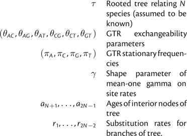
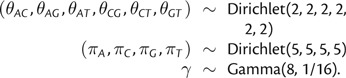
In our analyses, we assigned the following priors to the parameters of the phylogenetic model, assuming a known (fixed) rooted tree topology (τ):

The priors assigned to the parameters of the model of sequence evolution (GTR + Γ: including the exchangeability parameters, stationary frequencies, and the _γ_-shape parameter of the mean-one gamma distribution on among-site rate variation) are commonly employed priors in Bayesian phylogenetic analyses; we focus our attention on prior densities directly involved in estimating divergence times.
Birth–Death Prior on Node Ages
For this study, we assume node ages are distributed according to a birth–death process (Yule 1924, Kendall 1948, Yang and Rannala 1997) by applying the conditioned reconstructed process described by Gernhard (2008). This stochastic process models lineage diversification under a constant rate of speciation (λ) and a constant rate of extinction (μ) while assuming complete sampling of extant taxa. We treat the speciation and extinction rates as random variables, assigning a hyperprior to the net diversification rate (λ − μ) and the relative extinction rate (μ/λ), following Yang and Rannala (1997) and Gernhard (2008). Specifically, we assume
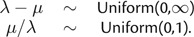
The birth–death process provides an appealing alternative to more general prior distributions on node ages, such as the flat Dirichlet (Kishino et al. 2001) or uniform (Lepage et al. 2007) priors, because it explicitly models lineage speciation and extinction (Yule 1924, Kendall 1948, Rannala and Yang 1996). However, work by Lepage et al. (2007) indicates that age estimates are sensitive to node time prior distributions and application of such priors should be conducted judiciously.
DPP on Branch Rates
The Dirichlet process is a stochastic process under which data elements are assumed to be clustered into distinct parameter classes (Ferguson 1973, Antoniak 1974). In phylogenetics, this model has recently been developed for modeling heterogeneity in the rate of amino acid replacement (Lartillot and Philippe 2004), among-site variation in the rates of nonsynonymous substitutions (Huelsenbeck et al. 2006), the distribution of concordant gene trees (Ané et al. 2007), and substitution rate variation across sites (Huelsenbeck and Suchard 2007). In the context of divergence time estimation, we use the DPP to model lineage-specific substitution rates by assigning branches to rate categories. Under this model, the substitution rate associated with each category is drawn from a single parametric distribution (_G_0) and partitioning of branches into specific rate categories is controlled by the concentration parameter (α). Here, we specify _G_0 such that the rate value for each class is drawn from a gamma distribution with constant values for the shape (s _G_0) and scale (β _G_0) parameters. The number of rate categories (k) and the number of branches assigned to each category both depend on the concentration parameter. The prior probability of a given number of substitution rate classes is conditional on the concentration parameter and the number of branches:
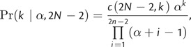
where c(·,·) is the Stirling number of the first kind. Small values of α lead to fewer categories and greater homogeneity of branch rates, whereas large values indicate increased partitioning. Thus, under the DPP, the rate values across all branches, (_r_1,…,r_2_N − 2), are dependent on α and _G_0, and the prior probability that any two branches share the same substitution rate is simply
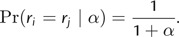
The global molecular clock (GMC) model (k = 1) and independent rates model (k = 2_N_ − 2) are both special cases of rate category partitions that can arise under a DPP. The calculation of the prior probability of a given number of rate categories is useful for model comparison using Bayes factors. The Bayes factor in favor of one model (_k_1) versus an alternative model (_k_2) can be computed by dividing the posterior odds (for a given set of data, X) by the prior odds (Kass and Raftery 1995):
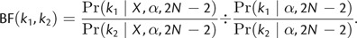
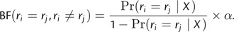
Thus, under the DPP on lineage-specific substitution rates, Bayes factors can be used to compare the relative support for two different values of k or to evaluate the evidence in favor of the GMC (k = 1) or the independent rates model (k = 2_N_ − 2). Additionally, Bayes factors can be calculated to assess the support for two branches sharing the same rate (Huelsenbeck and Andolfatto 2007):
When applying the Dirichlet process model to any problem, consideration must be given to the value of the concentration parameter (α). A hierarchical Bayesian approach provides a means for accommodating uncertainty in the value of α (Escobar and West 1995, Dorazio 2009), and this is accomplished by placing a second-order prior distribution, or “hyperprior,” on this prior parameter. Escobar and West (1995) specify a gamma-distributed hyperprior on α, which leads to full conditional distributions that can be easily sampled using Gibbs sampling. Following their example, we assume that _α_∼Gamma(s α,β α), where s α and β α are the shape and scale parameters of the gamma distribution, respectively, such that the expected value of the concentration parameter is: E(α) = s α β α. We parameterize the hyperprior on α by first specifying a prior mean number of rate categories, which leads to an approximation of E(α) based on
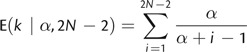
(Liu 1996, McAuliffe et al. 2006, Jara et al. 2007). Thus, the gamma-distributed hyperprior on the concentration parameter is parameterized when provided with a shape parameter value (s α) and a prior mean number of rate categories for a given data set. This hierarchical approach frees the user from the responsibility of specifying a precise value for α, while accounting for uncertainty in the degree of clustering. Moreover, a variety of studies applying the gamma hyperprior have shown that data are typically very informative about the value of the concentration parameter and the number of parameter categories (West et al. 1994, Escobar and West 1995, Gelfand et al. 2005, Dorazio 2009). Analyses under the Dirichlet process model can also be sensitive to the characterization of the base distribution parameter (McAuliffe et al. 2006), and it is possible to place additional hyperpriors on the parameters of _G_0 (Teh et al. 2006). However, this approach requires some further investigation into appropriate hierarchical models and can be computationally complex; therefore, we did not apply hyperprior distributions to _G_0 in the present study.
The DPP on lineage-specific substitution rates and the birth–death prior on speciation times were implemented in the C++ program DPPDiv, available at http://cteg.berkeley.edu/software.html. In this program, the likelihood is calculated using the sum product algorithm (Gallager 1962, Gallager 1963, Felsenstein 1981). We use Markov chain Monte Carlo (MCMC) sampling to approximate the posterior distributions of the various parameters and hyperparameters (Metropolis et al. 1953, Hastings 1970) and obtain estimates of branch rates and divergence times. The proposal mechanism for updating the lineage-specific substitution rates under the DPP is Algorithm 8 described by Neal (2000) and implemented in other phylogenetic methods employing this prior (Huelsenbeck and Suchard 2007). This approach uses Gibbs sampling to update the rate class assignments for each branch by evaluating the relative probabilities of all possible reassignments to existing classes and to placement in new auxiliary classes (Neal 2000). The number of auxiliary categories is fixed at four in this implementation to mitigate the computational burden of each Dirichlet process update while still adequately searching parameter space. An additional update is performed to propose changes to the rate values associated with every existing category using a rate multiplier.
The program was tested for correctness by performing numerous analyses on “empty” data sets so that the Markov chains sampled only from prior distributions. Distributions of MCMC samples obtained from these runs were examined in the program Tracer v1.5 (Rambaut and Drummond 2009), and the mean values of the various parameters were compared with expected values.
Materials and Methods
We evaluated the performance of Bayesian estimation of divergence times under the DPP on lineage-specific substitution rates by analyzing a previously published alignment of nucleotide sequences and using simulated data. We compared the accuracy and power of node time and branch rate estimates under the DPP with two alternative priors (both special cases of the Dirichlet process model): the GMC and gamma-distributed independent rates (IR-G).
Simulations: Data Generation
We simulated 100 ultrametric phylogenetic trees with branching times under a constant-rate birth–death process (Kendall 1948). These trees were generated using a general sampling approach described in Hartmann et al. (2010) and Stadler (2011) with a speciation rate equal to 0.01 and an extinction rate of 0.009. For each simulated birth–death tree, we produced six molecular data sets under different models of substitution rate variation. Lineage-specific substitution rates were applied to each simulated tree producing model phylogenies for generating nucleotide alignments such that the branch lengths were in units of expected number of substitutions per site (fig. 1). In all six trees, the rate of substitution at the root of the tree was drawn from a gamma distribution with a shape parameter equal to 2.0 and an inverse scale parameter of 4.0, so that the expected rate is equal to 0.5: r_2_N − 1∼ Gamma(2,1/4).
FIG 1.

An example of substitution rate models for a single simulation replicate. A birth–death tree was used to generate branch lengths in units of substitutions/site under six different models: the global molecular clock (GMC), local molecular clock (LMC), compound Poisson process model (CPP), log-normally distributed autocorrelated rates (AR-LN), gamma-distributed uncorrelated rates (IR-G), and the Dirichlet process model (DPPR). Note that the global clock tree (GMC) is proportional to the simulation tree, although the branches are scaled by the clock rate
Global Molecular Clock
Under a GMC, all branches share the same substitution rate (Zuckerkandl and Pauling 1962). Branch lengths were simply the product of the rate at the root (r_2_N − 1) and the branch time, resulting in trees with an average total tree length (the sum of all branch lengths) of 2.023 expected substitutions/site (fig. 1: GMC).
Local Molecular Clocks
An LMC model assumes that adjacent lineages are more likely to share the same substitution rate, and rate shifts occur relatively infrequently on the tree (Hasegawa et al. 1989, Kishino and Hasegawa 1990, Yoder and Yang 2000, Yang and Yoder 2003, Drummond and Suchard 2010). We generated branch rate heterogeneity under this model by traversing the tree from the root to the tips. At each node, a rate shift occurred with a probability equal to 0.15. If the event resulted in a rate shift, a new rate was drawn for the lineage from the initial gamma distribution; otherwise, the rate associated with the branch was equal to that of the parent lineage. The 100 trees simulated under this model had an average total tree length (the sum of all branch lengths) of 2.075 expected substitutions/site (fig. 1: LMC).
Compound Poisson Process
Huelsenbeck et al. (2000) described a complex model of lineage-specific substitution rate variation, in which rate changes occur along a branch according to a Poisson process. At each rate change event, a new rate is obtained by multiplying the previous rate by a gamma-distributed random variable. For a given branch, rate change events were sampled from a Poisson distribution on the time duration of the branch. We assumed that the expected number of rate changes along a single path from the root of the tree to an extant descendant was equal to 2. At each rate change, a new rate was obtained by multiplying the preceding rate by a gamma-distributed random number. Following Huelsenbeck et al. (2000), this gamma distribution was parameterized such that the expected value of the logarithm of the rate multiplier is equal to 0. Accordingly, rate multipliers were sampled from a gamma distribution with a shape parameter equal to 20 and a scale parameter of e_ψ_(20), where ψ is the logarithmic derivative of the Gamma function (Huelsenbeck et al. 2000). The weighted average of rates along the branch was calculated to obtain the branch length; trees generated under this model had an average total tree length of 2.019 expected substitutions/site (fig. 1: CPP).
Lognormally Distributed Autocorrelated Rates
Change in the rate of substitution occurs gradually over the tree and closely related lineages have similar rates under the model presented by Thorne et al. (1998) and Kishino et al. (2001). At each descendant node, a new rate was drawn from a lognormal distribution parameterized such that the expected value of the new rate is equal to the parent rate and the variance is equal to the product of the time duration between the two nodes and a variance parameter, which was fixed to 0.4 (Kishino et al. 2001). The substitution rate applied to each branch was the average of the beginning and ending rates and resulted in trees with a significant signal of rate autocorrelation and an average total tree length equal to 1.731 expected substitutions/site (fig. 1: AR-LN).
Gamma-Distributed Independent Rates
Lineage-specific rates are uncorrelated when the rate assigned to each branch is independently drawn from an underlying distribution. This model was first described by Drummond et al. (2006), and variants of the uncorrelated rates model are commonly used for divergence time estimation in the program BEAST (Drummond and Rambaut 2007). For our simulations, the rates associated with each branch were drawn from the distribution Gamma(2,1/4) and produced a set of trees with an average total tree length of 1.925 expected substitutions/site (fig. 1: IR-G).
Dirichlet Process Prior Rates
Under this model, rate values are assigned to lineages of the tree according to the DPP model (Ferguson 1973, Antoniak 1974). Simulation under the Dirichlet process was performed by selecting the first branch and assigning it to a new rate category. Subsequent branches on the tree were placed in an existing category with a probability proportional to the number of branches already present in that category or assigned to a new rate category with a probability proportional to the Dirichlet process concentration parameter (α = 1.28). The value of α chosen for these simulations leads to approximately four branch rate categories for a tree with 10 taxa (for our simulations, the median was 4, ranging between 2 and 6 rate classes). The rate value assigned to each category was drawn from Gamma(2,1/4). Lineage-specific rates generated under this model are not autocorrelated and distantly related branches can share the same substitution rate. Under the Dirichlet process model (DPP-R) model, the 100 trees had an average total tree length of 1.932 expected substitutions/site (fig. 1: DPP-R).
Each tree simulated under the birth–death process was used to create six different phylograms using the models of substitution rate variation described above. With the 600 model phylogenies, we simulated DNA sequence alignments, each with 2,000 nucleotides, under the GTR + Γ model of sequence evolution (Tavaré 1986, Yang 1994) using the program Seq-Gen (Rambaut and Grassly 1997). The parameter values for the GTR + Γ model (including the exchangeability parameters, stationary frequencies, and the _γ_-shape parameter of the mean-one gamma distribution on among-site rate variation) were drawn from the following distributions for each data set simulation:
Simulations: Analysis
We analyzed each of the 600 simulated data sets (100 replicate tree topologies × 6 rate models) under three different prior models on lineage-specific substitution rate variation: the DPP, the GMC, and independent branch rates. For each analysis, we assumed the GTR + Γ model of sequence evolution (the true model) and a birth–death prior on the branching times. All analyses were run for 2 million iterations, sampling every 100 steps. To rule out possible effects resulting from uncertainty in estimating phylogenetic relationships, we fixed the topology to that of the true tree for every run. We evaluated the performance of priors on lineage-specific substitution rates in the absence of node calibrations, thus, all divergence times are estimated relative to the age of the root.
In our implementation of Bayesian divergence time estimation, a gamma distribution is used as a prior on lineage-specific substitution rates. For the three types of analyses performed in this study, we fixed the parameters of this prior distribution to match the distribution used throughout our simulations: Gamma(2,1/4). Specifically, this distribution is applied as a prior on the single rate under the GMC, on individual branch rates under the independent rates model, and on the category-specific rates in the DPP model (_G_0). The analyses conducted using the DPP used a gamma-distributed hyperprior on the concentration parameter with a mean value of 1.9305 and a variance of 1.8634 (which leads to a prior mean number of rate categories of 5).
Given that our study design involved 600 simulated data sets and thousands of estimated parameters, it was not feasible to assess convergence of all MCMC analyses, and it is possible that some of the runs failed to reach convergence. Nevertheless, since these models are compared under identical implementations, the results of our analyses can improve our understanding of the relative performance of the three models.
Simulations: Accuracy Assessment
Analyses of simulated data provide straightforward ways to assess the performance and power of Bayesian inference methods. Statistics for every parameter sampled over the course of the MCMC run can be calculated and compared with the true simulated values. Specifically, we calculated the mean and median for the height of each node and each branch rate estimated in our analyses using the tools available in DendroPy (Sukumaran and Holder 2010). Additionally, we approximated the 95% highest posterior density interval by computing the 95% credible interval (CI) for each MCMC sample. We evaluated the accuracy of node height and rate estimates by computing coverage. The coverage probability for a method is the proportion of replicates for which the 95% CIs contain the true values. Coverage probabilities can be computed across several nodes within a single analysis or across simulation replicates. For our simulations, we computed coverage probabilities for node heights and branch rates under each of our priors on substitution rate variation. Analyses with coverage probabilities approximately equal to 0.95 are considered unbiased and robust estimators. Additionally, for each estimate of branch rate, we calculated the percentage error to quantify accuracy:

where the absolute difference of the estimated (ri^) and true (r i) rates for a given branch (i) is divided by the true branch rate and multiplied by 100%. Some estimators can sacrifice power for accuracy, however. Thus, we measured the power of an estimate by calculating the widths of the 95% CIs. Large 95% CIs indicate reduced power.
Analysis of Biological Data
We applied the DPP on lineage-specific substitution rate variation to an empirical alignment of two mitochondrial genes (cytochrome-b and cytochrome oxidase subunit II) presented in a paper by Yang and Yoder (TreeBASE study ID S1021 2003). This data set includes sequences for several primate species with a specific emphasis on “cute-looking” mouse lemurs in the genus Microcebus. Additionally, this alignment contains several sequences outside of Primates as outgroups. In their study, Yang and Yoder (2003) applied a maximum likelihood method with a priori-specified LMCs and a Bayesian method that assumed log-normally distributed autocorrelated rates (AR-LN) (Thorne et al. 1998, Kishino et al. 2001, Thorne and Kishino 2002) to estimate divergence times for this group. Based on unconstrained branch length estimates, three substitution rate categories were identified and placed on the Simiiformes clade (represented in this data set by Callithrix, Macaca, Pongo, Gorilla, Pan, and Homo), the Microcebus clade, and the remaining lineages, respectively, for analyses assuming LMCs (Yang and Yoder 2003).
Using the topology and upper and lower bounds on calibrated nodes presented in Yang and Yoder (2003), we estimated branch-specific rates and divergence times under the DPP for these data. We parameterized the gamma-distributed hyperprior on α by setting specific values for the prior mean number of rate categories (6.0) and the shape parameter (s α = 2.0), so that the expected value of the concentration parameter was equal to 1.396, with a variance of 0.974 (β α = 0.698). Unlike the analyses of Yang and Yoder (2003), which employed the Jukes–Cantor (Jukes and Cantor 1969) or F84 + Γ (Hasegawa et al. 1985, Felsenstein 1993, Yang 1994) models of sequence evolution, we assumed a GTR + Γ model for this study. Uniform distributions with soft bounds were used as priors on fossil-calibrated nodes (Yang and Rannala 2006). We ran six independent and identical MCMC chains, each for 3 million iterations. The last 1 million samples from each run were combined after convergence was assessed by evaluating the marginal distributions and effective sample sizes of relevant parameters in the program Tracer v1.5 (Rambaut and Drummond 2009).
In order to evaluate the strength of support for the GMC or independent rates models, we ran two separate analyses, one with α fixed to 0.002 (which leads to approximately 1 expected rate category) and another with α set to 240.7 (approximately 59 expected rate categories). Moreover, sensitivity to the hyperprior distribution on the Dirichlet process concentration parameter was evaluated by conducting additional runs with different expected values of α. Each analysis applied a gamma-distributed hyperprior on α with a shape parameter equal to 2.0, and the scale parameter was manipulated so that the expected value of alpha, E(α), was equal to 0.476, 1.396, 9.184, or 240.7. Each of these values respectively corresponds to an (approximate) expected number of substitution rate categories (k): 3, 5, 18, and 59, covering a wide range of values for α. Comparisons of the marginal densities of prior and posterior samples of k were evaluated to determine if the data are informative about the value of α and the number of rate categories.
Results and Discussion
Simulations
Estimates of branch-specific rates under the DPP are compared with the true branch rates in figure 2. These results show that as variation in the rate of substitution over the tree increases, the variation in the error of branch rate estimates also increases (fig. 2). However, on average, estimates of branch-specific substitution rates are accurate and unbiased under the DPP.
FIG 2.
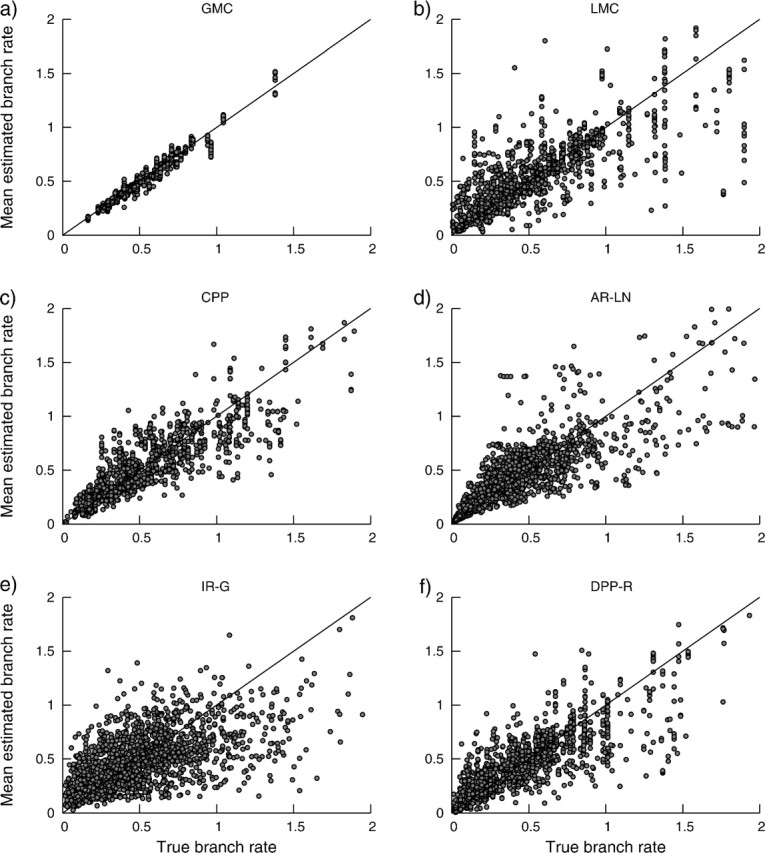
The posterior mean lineage-specific rates estimated under the DPP model compared with the true branch rates for data sets with substitution rates generated under different models of among-lineage rate variation: (a) the GMC, (b) LMCs, (c) the CPP, (d) AR-LN, (e) IR-G, and (f) uncorrelated rates generated under the Dirichlet process. Each point represents a single mean branch rate estimate across all simulation replicates. The solid line indicates the line of equality.
For each of the three different types of analyses, we calculated the coverage probability for branch-specific substitution rate estimates across all replicates for the six different rate variation models used for simulation (table 1). Analyses assuming either a DPP or independent rates relaxed-clock models produced estimates of branch rates with high coverage probabilities for all simulation treatments compared with strict clock analyses (table 1). When variation in lineage-specific substitution rate is introduced, analyses employing a GMC result in a high proportion of branches, in which the true rate is not contained within the 95% CI. Predictably, both the DPP and the independent rates model returned high coverage for rate estimates when the simulation model matched that of the analysis model (DPP-R/DPP and IR-G/independent rates, respectively).
Table 1.
The Coverage Probabilities for Branch Rate Estimates Across All Simulation Replicates
| Rate Variation | Independent | Global | |
|---|---|---|---|
| Simulation Model | DPP | Rates | Clock |
| Global molecular clock (GMC) | 0.9878 | 0.9633 | 0.9200 |
| Local molecular clocks (LMC) | 0.9078 | 0.9078 | 0.3978 |
| Compound Poisson process (CPP) | 0.8067 | 0.8611 | 0.3178 |
| Autocorrelated log-normal (AR-LN) | 0.8006 | 0.8444 | 0.2572 |
| Gamma-distributed independent rates (IR-G) | 0.8739 | 0.9389 | 0.1256 |
| Dirichlet process prior rates (DPP-R) | 0.9117 | 0.9078 | 0.2917 |
Table 1 also shows that the coverage probabilities for branch rate estimates are somewhat higher for analyses assuming an independent rates model when data are simulated under the compound Poisson process model (CPP) or AR-LN. However, when examining the percent error of branch rate estimates for our simulations (fig. 3), we found that the estimates produced by the independent rates model are less accurate, on average, than rate estimates under the Dirichlet process or global clock models for all simulation models except for IR-G. This discrepancy is due to the fact that analyses under our implementation of the independent rates model result in branch rate estimates with very large 95% CIs compared with those produced by the DPP or global clock analyses (fig. 4). In figure 4, we binned the true branch rates across all simulation replicates, so that each bin contained 200 values. For each bin, we calculated the average 95% CI size for each of the three different rate variation priors. This figure illustrates the relatively low power of the independent rates model. Furthermore, figure 4 demonstrates the flexibility of the DPP on lineage-specific substitution rates. This model behaves similarly to the global clock model when the data are simulated under a single rate, and conversely, it performs comparably with the independent rates model when data are generated under uncorrelated substitution rates. It is important to note that the precision of the independent rates model can be improved if the underlying gamma distribution has low variance, provided the prior is unbiased. Alternately, a hyperprior applied to the parameters of the gamma distribution from which rates are independently drawn can improve the power of estimates under this model, an approach, although not implemented here, that can be applied to variants of the independent rates model available in current versions of the program BEAST (Drummond and Rambaut 2007). Moreover, in cases in which the rate distribution is unknown, it may be best to apply a model averaging approach, where branch rates are estimated under a set of different models (Li and Drummond 2011).
FIG 3.

The percentage error calculated for branch rate estimates under the DPP (gray), the GMC (white), and the independent rates model (cross-hatched). Box plots indicate each sample minimum, lower quartile, median, upper quartile, and sample maximum of the percentage error in branch rate estimates across all simulation replicates for each model of substitution rate variation: the GMC, LMC, CPP, AR-LN, IR-G, and DPP-R.
FIG 4.

The sizes of branch rate 95% CIs from analyses under the DPP (•), GMC (□), and independent rates models (×) plotted against the true branch rates. Analyses were performed on data sets with substitution rate variation generated under six different models: (a) the GMC, (b) LMCs, (c) the CPP, (d) AR-LN, (e) IR-G, and (f) uncorrelated rates generated under the Dirichlet process. For each comparison, the true branch-specific rates were binned, so that each bin contained 100 rate values and the average 95% CI range was calculated for each bin.
A somewhat different pattern emerges upon evaluation of the coverage probabilities for node height estimates (table 1). We found that node height estimates under the DPP resulted in higher coverage probabilities, compared with the two alternative priors, for all but one of our simulation models. For data simulated under uncorrelated IR-G, the analyses employing the independent rates model out performed the DPP (table 2). These results were examined further by comparing coverage probabilities for node height estimates to the true relative node ages (fig. 5). For each of the three different analyses, we binned the true relative node heights so that each contained 100 nodes, then computed the coverage probability for each bin. These results show that the true node height was most often contained by the 95% CI for very young nodes (fig. 5). This effect is particularly evident for analyses under the global clock model. With the exception of data generated under the IR-G model, assuming a DPP on substitution rate variation provided node age estimates with greater coverage relative to the independent rates model. Moreover, this effect was not a result of larger 95% CIs (fig. 6). In figure 6, we compare the sizes of the 95% CIs with the true relative node heights. We observed that, for each of the six different simulation models, analyses under the independent rates model produce larger 95% CIs for node height estimates compared with analyses under the Dirichlet process (fig. 6). Thus, the greater coverage probabilities for the Dirichlet process prior observed in table 2 and figure 5 are not coupled with a reduction in power compared the independent rates model.
Table 2.
The Coverage Probabilities for Node Height Estimates across All Simulation Replicates
| Rate Variation | Independent | Global | |
|---|---|---|---|
| Simulation Model | DPP | Rates | Clock |
| GMC | 0.9888 | 0.9513 | 0.9650 |
| LMC | 0.8812 | 0.8400 | 0.4850 |
| CPP | 0.8013 | 0.7700 | 0.5038 |
| AR-LN | 0.7425 | 0.6987 | 0.4363 |
| IR-G | 0.8712 | 0.9537 | 0.3025 |
| DPP-R | 0.9337 | 0.8337 | 0.4788 |
FIG 5.
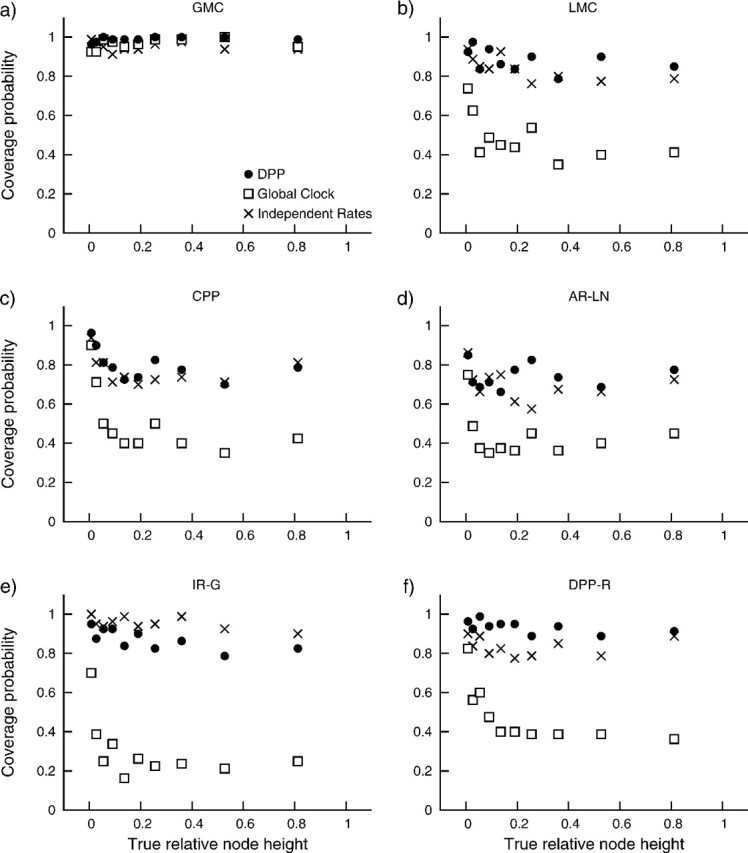
The proportion of node height estimates where the true value was sampled within the 95% CI (coverage probability) for analyses assuming the DPP (•), global clock (□), and IR-G (×) models compared with the true relative node heights. Coverage probabilities are presented for data generated under each rate variation model: (a) the GMC, (b) LMCs, (c) the CPP, (d) AR-LN, (e) IR-G, and (f) uncorrelated rates generated under the Dirichlet process. For each comparison, the true node heights were binned, so that each bin contained 100 nodes and the coverage probability was calculated for each bin.
FIG 6.
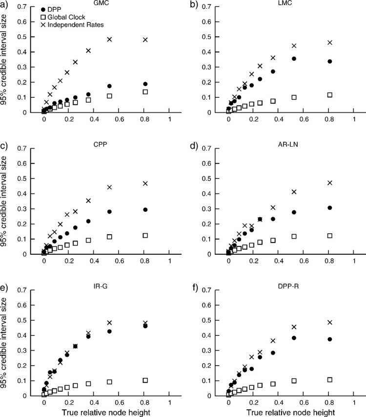
The sizes of node height 95% CIs produced by analyses under the DPP (•), global clock (□), and IR-G (×) models compared with the true relative node heights. Analyses were performed on data sets with substitution rate variation generated under six different models: (a) the GMC, (b) LMCs, (c) the CPP, (d) AR-LN, (e) IR-G, and (f) uncorrelated rates generated under the Dirichlet process. For each comparison, the true node heights were binned, so that each bin contained 100 nodes and the average 95% CI width was calculated for each bin.
Overall, we found that divergence time estimation under the DPP results in reliable estimates of branch rate and node age compared with the independent rates and global clock models across a range of different simulation models for substitution rate variation. Additionally, when the data were simulated under models that generated distinct rate classes, specifically the LMC and DPP-R models, analyses under the DPP accurately identified the true number of rate categories, with coverage probabilities of 0.94 and 0.97, respectively. Furthermore, inference under the DPP provides a way to summarize the estimates of branch rate and identify latent rate classes that may be present in the data. Huelsenbeck and Andolfatto (2007) describe a number of approaches to summarizing MCMC samples from analyses assuming a DPP. One such method identifies amean partitioning strategy that involves calculating partition distances (Gusfield 2002). In the context of divergence time estimation, this is done by identifying the set of branch partitions that minimizes the squared distance to all the partition sets in the MCMC sample. Figure 7 illustrates this using a single replicate from the simulations under the LMC model. The true tree with branch lengths proportional to the expected number of substitutions per site shows three different rate categories: 0.02 (blue branches), 0.7 (black branches), and 1.2 substitutions/site/time (red branches; fig. 7a). Divergence time estimation analysis, assuming a DPP on among-lineage substitution rate variation, was conducted on a molecular data set generated on the tree in figure 7a. The mean partition set was computed after a burn-in of 1,000,000 iterations. Figure 7b shows a plot of the mean estimated rate and 95% CI for each branch. The three different colors indicate the branch rate categories in the mean partition set identified by the Dirichlet process analysis: a slow rate (blue lines), a moderate rate (black lines), and a high rate (red lines). The analysis of this data set under the DPP correctly identified three latent rate classes. Our analysis also correctly partitioned all but one of the branches (branch number 3) into their respective rate categories. The single incorrect assignment was a particularly short branch and the 95% CI overlaps with rate estimates for both the moderate and high rate categories, indicating uncertainty in the rate estimate for this branch. In spite of the misassignment of this branch, the analysis provided accurate age estimates for both nodes subtending it (fig. 7c). The branch lengths in the tree in figure 7c display the mean branch times estimated under the DPP, with the gray bars representing the 95% CIs for the age of each node and the yellow rectangles indicate the true relative node ages. This example illustrates the capacity of divergence time estimation under the DPP to produce reliable estimates of speciation times. Moreover, this method provides a unique way to summarize the analysis and identify LMCs or latent rate classes.
FIG 7.
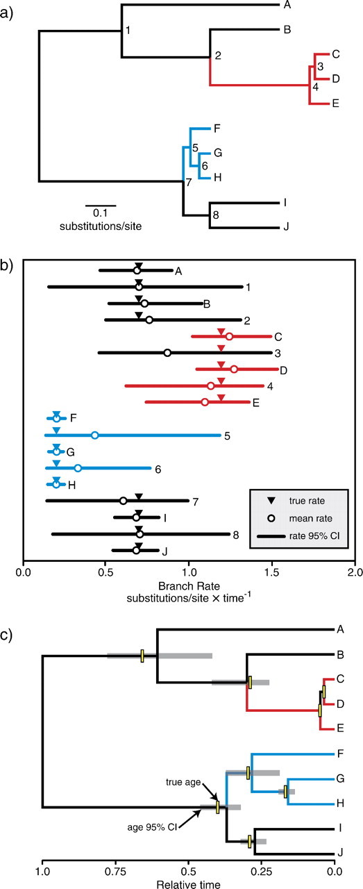
An example of the results yielded from divergence time analysis under the DPP. (a) The true tree topology and branch lengths used to simulate the data set, with branch rates generated under a local clock model. The branches are colored according to their rate (black: 0.7; blue: 0.02; and red:1.2 substitutions/site/time). Terminal branches/taxa are labeled with letters (A–B) and internal branches/nodes are labeled with numbers (1–8). (b) The estimates of lineage-specific substitution rate (in units of substitutions/site/time) under the Dirichlet process model. Each estimate is labeled according to its corresponding branch in the tree (a) and colored according to the mean partition estimated under the DPP model. True rates for each branch are indicated with inverted triangles, mean rates sampled under the DPP model are represented with open circles, and 95% CIs are shown with lines. (c) The average relative node ages estimated under the DPP model. Gray bars indicate 95% CIs of node heights and each branch is colored according to the mean partition estimated under the DPP model. Yellow bars represent the true divergence time for each internal node.
The model we have presented is similar to the random-local clock (RLC) model of Drummond and Suchard (2010). The RLC model identifies rate changes over the tree and treats these events as random variables. One marked correspondence with the Dirichlet process model described here is that the GMC (0 rate changes) and the independent rates (2_N_ − 2 rate changes) models are nested within the RLC model. The DPP departs from the RLC model in that it clusters branches without regard to their position in the tree. This flexibility allows for identifying both LMCs and branch rate clusters that do not correspond to the topological structure of the data. The RLC model may, however, have comparable performance to the Dirichlet process model since it can approximate this pattern by proposing multiple rate shifts on the tree. Yet, we did not include this model in our comparisons since its current implementation (in BEAST v1.6; Drummond and Rambaut 2007) can induce long mixing times for some data sets (Drummond and Suchard 2010, Dornburg et al. 2011).
Biological Data
Consistent with the results of Yang and Yoder (2003), our analyses do not provide support for the strict molecular clock for the primate sequence data. When the concentration parameter was fixed to a very low value (0.002), Bayes factor analyses showed very strong support for values of k greater than 2. However, the Bayes factor in support of the single-rate model could not be calculated using the ratio of posterior odds to prior odds because k = 1 was never sampled by the MCMC algorithm after the initial burn-in. Likewise, when α was fixed to an extremely high value (240.7), values of k less than 68 were strongly supported by Bayes factors because partition sets with greater than 63 rate categories were never sampled. Although the results indicate strong support for the presence of lineage-specific substitution rate clusters in these data, Bayes factor analysis using marginal likelihoods would bolster these conclusions. The marginal likelihood is used to quantify the fit of a particular model to the data, and the Bayes factor is the ratio of the marginal likelihoods for two competing models. Recently introduced methods for approximating marginal likelihoods have made an important contribution to Bayesian hypothesis testing in phylogenetics (Lartillot and Philippe 2006, Fan et al. 2010, Xie et al. 2011). In their investigation of the diversification of the Hymenoptera, Ronquist et al. (Forthcoming) used the stepping stone method (Xie et al. 2011) to perform Bayes factor comparisons of three different relaxed-clock models: the independent gamma rates model also called the “white noise” model by Lepage et al. (2007), the CPP model (Huelsenbeck et al. 2000), and the AR-LN model (Thorne and Kishino 2002). They found that, despite signal for autocorrelation among branch-specific rates, Bayes factor comparisons favored the independent rates and the CPP models, which allow for abrupt changes in rates over the tree. In contrast, Lepage et al. (2007) used thermodynamic integration (Lartillot and Philippe 2006) to estimate marginal likelihoods and compute Bayes factors for three different data sets and showed that autocorrelated models outperformed uncorrelated models in every case. Although model comparison methods using Bayes factors provide powerful statistical tools for evaluating and understanding the properties of priors employed in phylogenetic analyses, due to the computational complexity of methods for calculating marginal likelihoods, these analyses were not performed for this study. However, we do believe that further investigation of the statistical fit of relaxed-clock models to biological data is an important direction for future work.
We found further support for lineage-specific rate partitions when comparing estimates of k under different hyperpriors on the _α_-concentration parameter. Figure 8 shows the probabilities of different values of k for samples from both the posterior (dark bars) and prior (light bars) distributions for each of the four analyses. Under each of the four different hyperpriors, the median value of k was 3, 5, 18, and 59, respectively. However, when the Markov chain sampled from the posterior distributions, the median value of k ranged only from 4 to 9 rate categories across the four different hyperpriors, indicating strong support for partitioning of lineages into rate clusters. Moreover, estimates of divergence times, rates, and branch partitions were not overtly influenced by the hyperprior on the concentration parameter. This prior sensitivity analysis showed that the data were distinctly informative about the number of rate clusters and robust to the parameterization of the hyperprior on α.
FIG 8.

The posterior and prior probabilities of the number of rate categories (k) for analyses on a primate data set with different expected values of the DPP concentration parameter (α). The histograms show the probability of values of k sampled by the MCMC algorithm when sampling from the posterior distribution (top, dark bars) or from the prior distribution (bottom, light bars). Four separate analyses were conducted, each with different parameterizations of the gamma-distributed hyperprior on α. The expected values of α are: (a) 0.476, (b) 1.396, (c) 9.184, and (d) 240.67. The median values of k and the 95% CIs are indicated for each E(α).
Figure 9 displays the phylogenetic relationships of the primate sequences presented in Yang and Yoder (2003) with branch lengths proportional to a) the expected number of substitutions/site estimated under the Dirichlet process model (ν i = r i t i) and b) the mean estimated substitution rate for each branch (r i). The branches in figure 9 are colored according to a) the mean partition categorization and b) the mean estimated branch rate (r i) estimated under the Dirichlet process model. Although our analyses also uncovered three distinct rate categories: a high rate (fig 9a: red branches), a moderate rate (fig 9a: black branches), and a low rate (fig 9a: blue branches), the rate class assignments did not match those of the LMCs described by Yang and Yoder (2003), which placed the simians in the highest rate category, Microcebus in the moderate (or next highest) category, and the remaining lineages in a lower rate category. Some of the highest rates were estimated for most of the Simiiformes lineages (fig. 9b), however, which is consistent with the high rate assigned to that clade by Yang and Yoder (2003).
FIG 9.

Branch rate estimates from an analysis of primate mitochondrial sequences. (a) The topology with branch lengths proportional to the number of expected substitutions per site with branches colored according to the mean partition estimated under the DPP. (b) The topology with branch lengths proportional to the mean rate estimated for each branch and colored according to a gradient where blue indicates the lowest rate and red indicates the highest. The subclades designated with specific rates by Yang and Yoder (2003) are highlighted with gray boxes. In their study, the Simiiformes had the highest rate and Microcebus had the next highest rate compared with the remaining lineages.
In spite of differences between the divergence time analyses conducted by Yang and Yoder (2003) and our study, we found that the majority of node age estimates resulting from the Dirichlet process analysis were consistent with the ages presented in the previous study (fig. 10). The tree in figure 10 shows the divergence time estimates obtained by Yang and Yoder (2003) using a maximum likelihood LMC method with calibrated nodes indicated by white circles. The gray bars in figure 10 represent the 95% CIs of node age estimated under the Dirichlet process model presented here. We show that almost all the 95% CIs estimated using the DPP overlap with the node ages obtained by Yang and Yoder (2003). This correspondence is likely a result of the low variation in substitution rates across the tree and the influence of informative priors on fossil-calibrated nodes.
FIG 10.

A comparison of divergence times estimated under different methods. The branch lengths are divergence times estimated by the previous study using a maximum likelihood local clock method (Yang and Yoder 2003). The gray bars show the node age 95% CIs obtained from the divergence time analysis using the DPP on rate variation presented in this study. White circles indicate nodes calibrated by the fossil age estimates presented in the original study.
Conclusions
Accurate estimates of species divergence times are essential for understanding many aspects of evolutionary biology, such as historical biogeography, rates of diversification, and variation in rates of molecular evolution. However, obtaining reliable divergence time estimates is confounded by the fact that both the rate of evolution and time affect sequence divergence in the same way. To tease apart the rate of substitution and time, we must adopt a model for the rates of sequence evolution and how these rates change across a tree. We have presented a flexible model for use as a prior on lineage-specific substitution rates in Bayesian divergence time estimation that performs well under a wide range of conditions. Additionally, MCMC samples under the DPP can be summarized using partition distances for identifying lineages that share similar properties.
The Dirichlet process model is not entirely analogous to a distinct biological model, and its adequacy for modeling evolutionary processes requires further investigation. In particular, some analyses under this model may be sensitive to the parameterization of the base distribution (_G_0) and the concentration parameter (Escobar and West 1995, McAuliffe et al. 2006). Additionally, this nonparametric model can have a tendency to induce clusters (Dunson 2009), particularly when the concentration parameter (α) is very small or when there are branches with very similar rates, thus explaining the lower coverage probabilities of age and rate estimates under the DPP when data are simulated under the IR-G model, compared with estimates resulting from analyses assuming an independent rates model. Thus, it is important to assess and parameterize prior distributions by sensitivity analysis (McAuliffe et al. 2006), and future work leading to the development and evaluation of hyperpriors applied to the parameters of the DPP is required. Moreover, it seems unlikely that processes of molecular evolution would agree “exactly” with the Dirichlet process model. For example, it may be more plausible that the rate of evolution will be inherited by descendants, and that the rate of sequence evolution can change along a lineage anagenetically. Both these complications may be modeled more naturally by the CPP model of Huelsenbeck et al. (2000). However, some evolutionary processes could generate patterns, in which the rate of evolution changes substantially in at least one daughter lineage. This might be the case if the effective population size is a strong determinant of the rate of substitution (e.g., if relaxed selection in small populations cause the neutral mutation rate to be higher in these populations). Speciation by the formation of peripheral isolates could induce such a pattern. Thus, the DPP might be an effective way to model sequence evolution in a group, in which there were several widespread species with large population sizes and several species with very restricted ranges. Nevertheless, even if the model does not realistically encapsulate all the complexities of sequence evolution, the DPP is capable of approximating patterns present in biological data and lends itself to efficient MCMC implementations. Furthermore, the model's ability to handle cases, in which the changes of rate are not well-described as a local clock imply that the model can offer an alternative perspective to many of the relaxed-clock models (e.g., CPP, local clocks, or autocorrelated rates) that do assume some form of inheritance of the rate of sequence evolution by daughter species. The independent rates approaches also share these advantages, but our simulations indicate that introducing a new rate parameter for each branch can result in a noticeable loss of power.
Acknowledgments
We thank Jeff Thorne, Marcy Uyenoyama, Asger Hobolth, Stéphane Guindon, and two anonymous reviewers for their helpful comments on this manuscript. This research was supported by National Science Foundation (NSF) postdoctoral fellowship in biological informatics DBI-0805631 awarded to T.A.H.; NSF grant DEB-0918791 and National Institute of Health grants GM-069801 and GM-086887 awarded to J.P.H.; and NSF grant DEB-0732920 awarded to M.T.H.
References
- Ané C, Larget B, Baum DA, Smith SD, Rokas A. Bayesian estimation of concordance among gene trees. Mol Biol Evol. 2007;24:412–426. doi: 10.1093/molbev/msl170. [DOI] [PubMed] [Google Scholar]
- Antoniak CE. Mixtures of Dirichlet processes with applications to non-parametric problems. Ann Stat. 1974;2:1152–1174. [Google Scholar]
- Dorazio RM. On selecting a prior for the precision parameter of the Dirichlet process mixture models. J Stat Plan Inference. 2009;139:3384–3390. [Google Scholar]
- Dornburg A, Brandley MC, McGowen MR, Near TJ. Relaxed clocks and inferences of heterogeneous patterns of nucleotide substitution and divergence time estimates across whales and dolphins (Mammalia: Cetacea) Mol Biol Evol. 2011;29:721–736. doi: 10.1093/molbev/msr228. [DOI] [PubMed] [Google Scholar]
- Drummond AJ, Ho SY, Phillips MJ, Rambaut A. Relaxed phylogenetics and dating with confidence. PLoS Biol. 2006:4, e88. doi: 10.1371/journal.pbio.0040088. [DOI] [PMC free article] [PubMed] [Google Scholar]
- Drummond AJ, Rambaut A. BEAST: Bayesian evolutionary analysis by sampling trees. BMC Evol Biol. 2007;7:214. doi: 10.1186/1471-2148-7-214. [DOI] [PMC free article] [PubMed] [Google Scholar]
- Drummond AJ, Suchard MA. Bayesian random local clocks, or one rate to rule them all. BMC Biol. 2010;8:114. doi: 10.1186/1741-7007-8-114. [DOI] [PMC free article] [PubMed] [Google Scholar]
- Dunson DB. Nonparametric Bayes local partition models for random effects. Biometrika. 2009;96:249–262. doi: 10.1093/biomet/asp021. [DOI] [PMC free article] [PubMed] [Google Scholar]
- Escobar MD, West M. Bayesian density estimation and inference using mixtures. J Am Stat Assoc. 1995;90:577–588. [Google Scholar]
- Fan Y, Wu R, Chen MH, Kuo L, Lewis PO. Choosing among partition models in Bayesian phylogenetics. Mol Biol Evol. 2010;28:523–532. doi: 10.1093/molbev/msq224. [DOI] [PMC free article] [PubMed] [Google Scholar]
- Felsenstein J. Evolutionary trees from DNA sequences: a maximum likelihood approach. J Mol Evol. 1981;17:368–376. doi: 10.1007/BF01734359. [DOI] [PubMed] [Google Scholar]
- Felsenstein J. Seattle (WA): University of Washington; 1993. PHYLIP (phylogeny inference package) Available from: http://evolution.genetics.washington.edu/phylip.html. [Google Scholar]
- Ferguson TS. A Bayesian analysis of some nonparametric problems. Ann Stat. 1973;1:209–230. [Google Scholar]
- Gallager RG. Low-density parity-check codes. IRE Trans Inf Theory. 1962;8:21–28. [Google Scholar]
- Gallager RG. Cambridge (MA): MIT Press; 1963. Low-density parity check codes. [Google Scholar]
- Gaut BA, Weir BS. Detecting substitution-rate heterogeneity among regions of a nucleotide sequence. Mol Biol Evol. 1994;11:620–629. doi: 10.1093/oxfordjournals.molbev.a040141. [DOI] [PubMed] [Google Scholar]
- Gelfand AE, Kottas A, MacEachern SN. Bayesian nonparametric spatial modeling with Dirichlet process mixing. J Am Stat Assoc. 2005;100:1021–1035. [Google Scholar]
- Gernhard T. The conditioned reconstructed process. J Theor Biol. 2008;253:769–778. doi: 10.1016/j.jtbi.2008.04.005. [DOI] [PubMed] [Google Scholar]
- Gusfield D. Partition-distance: a problem and class of perfect graphs arising in clustering. Inf Process Lett. 2002;82:159–164. [Google Scholar]
- Hartmann K, Wong D, Stadler T. Sampling trees from evolutionary models. Syst Biol. 2010;59:465–476. doi: 10.1093/sysbio/syq026. [DOI] [PubMed] [Google Scholar]
- Hasegawa M, Kishino H, Yano T. Dating the human-ape splitting by a molecular clock of mitochondrial DNA. J Mol Evol. 1985;22:160–174. doi: 10.1007/BF02101694. [DOI] [PubMed] [Google Scholar]
- Hasegawa M, Kishino H, Yano T. Estimation of branching dates among primates by molecular clocks of nuclear DNA which slowed down in Hominoidea. J Hum Evol. 1989;18:461–476. [Google Scholar]
- Hastings WK. Monte Carlo sampling methods using Markov chains and their applications. Biometrika. 1970;57:97–109. [Google Scholar]
- Huelsenbeck JP, Andolfatto P. Inference of population structure under a Dirichlet process model. Genetics. 2007;175:1787–1802. doi: 10.1534/genetics.106.061317. [DOI] [PMC free article] [PubMed] [Google Scholar]
- Huelsenbeck JP, Jain S, Frost SWD, Pond SLK. A Dirichlet process model for detecting positive selection in protein-coding DNA sequences. Proc Natl Acad Sci U S A. 2006;103:6263–6268. doi: 10.1073/pnas.0508279103. [DOI] [PMC free article] [PubMed] [Google Scholar]
- Huelsenbeck JP, Larget B, Swofford DL. A compound Poisson process for relaxing the molecular clock. Genetics. 2000;154:1879–1892. doi: 10.1093/genetics/154.4.1879. [DOI] [PMC free article] [PubMed] [Google Scholar]
- Huelsenbeck JP, Suchard M. A nonparametric method for accommodating and testing across-site rate variation. Syst Biol. 2007;56:975–987. doi: 10.1080/10635150701670569. [DOI] [PubMed] [Google Scholar]
- Jara A, Garcia-Zattera MJ, Lesaffre E. A Dirichlet process mixture model for the analysis of correlated binary responses. Comput Stat Data Anal. 2007;51:5402–5415. [Google Scholar]
- Jukes TH, Cantor CR. Evolution of protein molecules. In: Munro HN, editor. 1969. Mammalian protein metabolism. New York: Academic Press. p. 21–123. [Google Scholar]
- Kass RE, Raftery AE. Bayes factors. J Am Stat Assoc. 1995;90:773–795. [Google Scholar]
- Kendall DG. On the generalized “birth-and-death” process. Ann Math Stat. 1948;19:1–15. [Google Scholar]
- Kishino H, Hasegawa M. Converting distance to time: application to human evolution. Methods Enzymol. 1990;183:550–570. doi: 10.1016/0076-6879(90)83036-9. [DOI] [PubMed] [Google Scholar]
- Kishino H, Thorne JL, Bruno W. Performance of a divergence time estimation method under a probabilistic model of rate evolution. Mol Biol Evol. 2001;18:352–361. doi: 10.1093/oxfordjournals.molbev.a003811. [DOI] [PubMed] [Google Scholar]
- Lartillot N, Philippe H. A Bayesian mixture model for across-site heterogeneities in the amino-acid replacement process. Mol Biol Evol. 2004;21:1095–1109. doi: 10.1093/molbev/msh112. [DOI] [PubMed] [Google Scholar]
- Lartillot N, Philippe H. Computing Bayes factors using theromodynamic integration. Syst Biol. 2006;55:195–207. doi: 10.1080/10635150500433722. [DOI] [PubMed] [Google Scholar]
- Lepage T, Bryant D, Philippe H, Lartillot N. A general comparison of relaxed molecular clock models. Mol Biol Evol. 2007;24:2669–2680. doi: 10.1093/molbev/msm193. [DOI] [PubMed] [Google Scholar]
- Lepage T, Lawi S, Tupper P, Bryant D. Continuous and tractable models for the variation of evolutionary rates. Math Biosci. 2006;199:216–233. doi: 10.1016/j.mbs.2005.11.002. [DOI] [PubMed] [Google Scholar]
- Li WLS, Drummond AJ. Model averaging and Bayes factor calculation of relaxed molecular clocks in Bayesian phylogenetics. Mol Biol Evol. 2011 doi: 10.1093/molbev/msr232. doi:10.1093/molbev/msr232. [DOI] [PMC free article] [PubMed] [Google Scholar]
- Liu JS. Nonparametric hierarchical Bayes via sequential imputations. Ann Stat. 1996;3:911–930. [Google Scholar]
- McAuliffe JD, Blei DM, Jordan MI. Nonparametric empirical Bayes for the Dirichlet process mixture model. Stat Comput. 2006;16:5–14. [Google Scholar]
- Metropolis N, Rosenbluth AW, Rosenbluth MN, Teller AH, Teller E. Equation of state calculations by fast computing machines. J Chem Phys. 1953;21:1087–1092. [Google Scholar]
- Muse SV, Weir BS. Testing for equality of evolutionary rates. Genetics. 1992;132:269–276. doi: 10.1093/genetics/132.1.269. [DOI] [PMC free article] [PubMed] [Google Scholar]
- Neal RM. Markov chain sampling methods for Dirichlet process mixture models. J Comput Graph Stat. 2000;9:249–265. [Google Scholar]
- Rambaut A, Drummond AJ. University of Edinburgh; 2009. Tracer v1.5. Edinburgh (United Kingdom): Institute of Evolutionary Biology. Available from: http://beast.bio.ed.ac.uk/Tracer. [Google Scholar]
- Rambaut A, Grassly NC. Seq-Gen: an application for the Monte Carlo simulation of DNA sequence evolution along phylogenetic trees. Comput Appl Biosci. 1997;13:235–238. doi: 10.1093/bioinformatics/13.3.235. [DOI] [PubMed] [Google Scholar]
- Rannala B, Yang Z. Probability distribution of molecular evolutionary trees: a new method of phylogenetic inference. J Mol Evol. 1996;43:304–311. doi: 10.1007/BF02338839. [DOI] [PubMed] [Google Scholar]
- Rannala B, Yang Z. Inferring speciation times under an episodic molecular clock. Syst Biol. 2007;56:453–466. doi: 10.1080/10635150701420643. [DOI] [PubMed] [Google Scholar]
- Ronquist F, Klopfstein S, Vilhelmsen L, Schulmeister S, Murray DL, Rasnitsyn Forthcoming AP. A total-evidence approach to dating with fossils, applied to the early radiation of the Hymenoptera. Syst Biol. doi: 10.1093/sysbio/sys058. [DOI] [PMC free article] [PubMed] [Google Scholar]
- Sanderson MJ. A nonparametric approach to estimating divergence times in the absence of rate constancy. Mol Biol Evol. 1997;14:1218–1231. [Google Scholar]
- Sanderson MJ. Estimating absolute rates of molecular evolution and divergence times: a penalized likelihood approach. Mol Biol Evol. 2002;19:101–109. doi: 10.1093/oxfordjournals.molbev.a003974. [DOI] [PubMed] [Google Scholar]
- Stadler T. Simulating trees on a fixed number of extant species. Syst Biol. 2011;60:668–675. doi: 10.1093/sysbio/syr029. [DOI] [PubMed] [Google Scholar]
- Suchard MA, Weiss RE, Sinsheimer JS. Bayesian selection of continuous-time Markov chain evolutionary models. Mol Biol Evol. 2001;18:1001–1013. doi: 10.1093/oxfordjournals.molbev.a003872. [DOI] [PubMed] [Google Scholar]
- Sukumaran J, Holder MT. DendroPy: a Python library for phylogenetic computing. Bioinformatics. 2010;26:1569–1571. doi: 10.1093/bioinformatics/btq228. [DOI] [PubMed] [Google Scholar]
- Tajima F. Simple methods for testing molecular clock hypothesis. Genetics. 1993;135:599–607. doi: 10.1093/genetics/135.2.599. [DOI] [PMC free article] [PubMed] [Google Scholar]
- Tavaré S. Some probabilistic and statistical problems on the analysis of DNA sequences. Lectures Math Life Sci. 1986;17:57–86. [Google Scholar]
- Teh YW, Jordan MI, Beal MJ, Blei DM. Hierarchical Dirichlet processes. J Am Stat Assoc. 2006;101:1566–1581. [Google Scholar]
- Thorne J, Kishino H. Divergence time and evolutionary rate estimation with multilocus data. Syst Biol. 2002;51:689–702. doi: 10.1080/10635150290102456. [DOI] [PubMed] [Google Scholar]
- Thorne JL, Kishino H. In: Estimation of divergence times from molecular sequence data. Nielsen R, editor. 2005. Statistical methods in molecular evolution. New York: Springer. p. 235–256. [Google Scholar]
- Thorne J, Kishino H, Painter IS. Estimating the rate of evolution of the rate of molecular evolution. Mol Biol Evol. 1998;15:1647–1657. doi: 10.1093/oxfordjournals.molbev.a025892. [DOI] [PubMed] [Google Scholar]
- West M, Müller P, Escobar MD. Hierarchical priors and mixture models, with application in regression and density estimation. In: Smith AFM, Freeman P, editors. 1994. Aspects of uncertainty: a tribute to D. V. Lindley. Chichester (UK): Wiley. p. 363–386. [Google Scholar]
- Xie W, Lewis PO, Fan Y, Kuo L, Chen MH. Improving marginal likelihood estimation for Bayesian phylogenetic model selection. Syst Biol. 2011;60:150–160. doi: 10.1093/sysbio/syq085. [DOI] [PMC free article] [PubMed] [Google Scholar]
- Yang Z. Maximum likelihood estimation of phylogeny from DNA sequences when substitution rates differ over sites. Mol Biol Evol. 1993;10:1396–1401. doi: 10.1093/oxfordjournals.molbev.a040082. [DOI] [PubMed] [Google Scholar]
- Yang Z. Maximum likelihood phylogenetic estimation from DNA sequences with variable rates over sites: approximate methods. J Mol Evol. 1994;39:306–314. doi: 10.1007/BF00160154. [DOI] [PubMed] [Google Scholar]
- Yang Z, Rannala B. Bayesian phylogenetic inference using DNA sequences: a Markov chain Monte Carlo method. Mol Biol Evol. 1997;14:717–724. doi: 10.1093/oxfordjournals.molbev.a025811. [DOI] [PubMed] [Google Scholar]
- Yang Z, Rannala B. Bayesian estimation of species divergence times under a molecular clock using multiple fossil calibrations with soft bounds. Mol Biol Evol. 2006;23:212–226. doi: 10.1093/molbev/msj024. [DOI] [PubMed] [Google Scholar]
- Yang Z, Yoder AD. Comparison of likelihood and Bayesian methods for estimating divergence times using multiple gene loci and calibration points, with application to a radiation of cute-looking mouse lemur species. Syst Biol. 2003;52:705–716. doi: 10.1080/10635150390235557. [DOI] [PubMed] [Google Scholar]
- Yoder AD, Yang Z. Estimation of primate speciation dates using local molecular clocks. Mol Biol Evol. 2000;17:1081–1090. doi: 10.1093/oxfordjournals.molbev.a026389. [DOI] [PubMed] [Google Scholar]
- Yule GU. A mathematical theory of evolution, based on the conclusions of Dr. J. C. Wills, F. R. S. Philos Trans R Soc Lond B Biol Sci. 1924;213:21–87. [Google Scholar]
- Zuckerkandl E, Pauling L. In: Molecular disease, evolution, and genetic heterogeneity. Kasha M, Pullman B, editors. 1962. Horizons in biochemistry. New York: Academic Press. p. 189–225. [Google Scholar]