Interactive Prostate Shape Reconstruction from 3D TRUS Images (original) (raw)
. Author manuscript; available in PMC: 2017 Dec 21.
Published in final edited form as: J Comput Des Eng. 2014 Dec 18;1(4):272–288. doi: 10.7315/JCDE.2014.027
Abstract
This paper presents a two-step, semi-automated method for reconstructing a three-dimensional (3D) shape of the prostate from a 3D transrectal ultrasound (TRUS) image. While the method has been developed for prostate ultrasound imaging, it can potentially be applicable to any other organ of the body and other imaging modalities. The proposed method takes as input a 3D TRUS image and generates a watertight 3D surface model of the prostate. In the first step, the system lets the user visualize and navigate through the input volumetric image by displaying cross sectional views oriented in arbitrary directions. The user then draws partial/full contours on selected cross sectional views. In the second step, the method automatically generates a watertight 3D surface of the prostate by fitting a deformable spherical template to the set of user-specified contours. Since the method allows the user to select the best cross-sectional directions and draw only clearly recognizable partial or full contours, the user can avoid time-consuming and inaccurate guesswork on where prostate contours are located. By avoiding the usage of noisy, incomprehensible portions of the TRUS image, the proposed method yields more accurate prostate shapes than conventional methods that demand complete cross-sectional contours selected manually, or automatically using an image processing tool. Our experiments confirmed that a 3D watertight surface of the prostate can be generated within five minutes even from a volumetric image with a high level of speckles and shadow noises.
Keywords: Shape Reconstruction, Prostate, TRUS, Ultrasound, Image Processing
1 Introduction
The three-dimensional (3D) shape data of the prostate plays a key role in surgical interventions for diagnosing and treating prostate cancer, including biopsy, brachytherapy, high-frequency ultrasound (HIFU), and cryosurgery. For example, the prostate volume has been used in conjunction with prostate-specific antigen (PSA) for cancer diagnosis, and this volume can be calculated more accurately from 3D shape data than by using planimetry measurements (i.e., cross-sectional imaging across a plane of the prostate). The 3D-shape data is pivotal also in the pre-surgical planning, intra-operative image-based guidance, and post-surgical monitoring. In brachytherapy and cryosurgery, planning the placement of radioactive seeds or cryoprobes is a layout/coverage optimization problem that requires the 3D-shape data of the prostate. For HIFU, planning the sequential application of localized heating is a coverage optimization problem of a different kind that essentially requires the same 3D-shape data of the organ.
In addition to the conventional usage for cancer diagnosis and therapy, the 3D prostate-shape data can also be used in a computer-assisted cryosurgical training system. Based on the previous work on the thermal simulation of a cryosurgical procedure and cryoprobe layout optimization [1,2], the current research team has been building a computer-assisted trainer for cryosurgeons [3]. In this system, the 3D-shape data of the prostate is necessary for the visualization of the anatomy and cryoprobes, the calculation of the temperature distribution during a cryosurgical procedure, and the visualization of frozen regions against the target region.
In order to generate the 3D-shape data of the prostate accurately and efficiently for the computer-assisted training system for cryosurgery, a two-step semi-automated method has been developed. The proposed method takes as input a 3D transrectal ultrasound (TRUS) image – a set of parallel 2D cross-sectional images positioned in 3D space – and generates a 3D surface model of the prostate. 3D TRUS images can be generated by translating or rotating a 1D ultrasound transducer along an axis [4]. The 3D TRUS images used in this study were generated by Fenster and co-workers using a proprietary imaging system [5]. To make the output 3D-shape data suitable for the thermal simulation performed in the computer-assisted training system, the 3D-shape data must be watertight.
The comprehensibleness of our input 3D TRUS image ranges from low to medium due to noises such as speckles and shadows, as shown in Fig. 1. Poor image quality is a common weakness of ultrasound imaging, compared to magnetic resonance imaging (MRI) and computerized tomography (CT). Although MRI and CT images are clearer and more comprehensible, those imaging modalities are more time-consuming and expensive, and U.S. medical insurance companies typically do not reimburse for them. TRUS imaging is thus the choice of practice, which is used as input for our 3D prostate-shape generation. The proposed two-step method for reconstructing 3D shapes is specifically designed to work well with low quality TRUS images, where only partial prostate contours are comprehensible. The first step of the proposed method relies upon the user’s partial contour specification – the user is asked to select 10–15 easier-to-comprehend images, on which the user specifies partial or full contours. This can be completed within several minutes. Then, a final watertight 3D prostate shape is automatically generated within 20–30 seconds by fitting a deformable template shape to the specified contours.
Figure 1.
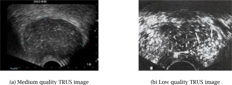
Typical TRUS images – part of an image is often not comprehensible due to speckle and shadow noises.
The proposed method is simpler and quicker than the conventional semi-manual method that requires the user to specify a set of complete closed contours in many more images, even when some images may be of poor quality. Figure 2 shows an example of such a conventional method of 3D shape generation using a commercial product, 3D Doctor [6]. The input was a 3D image consisting of 69 2D TRUS images. It took over 30 minutes for the user to specify a closed full contour for each of the 69 images. The system then created a 3D watertight shape automatically by joining adjacent cross-sectional contours, as illustrated in Figure 2(b). Although this commercial product offers an automated contour generation based on manually specified contours on several images, the method did not work well for our 3D image due to its poor image quality. The final 3D shape is not smooth due to inconsistent contour specifications on adjacent cross-sectional images. While the output shape captures the general size and shape of the prostate, the shape is not natural due to the noisy surface texture caused by non-coherent contour specification, making the 3D shape data unsuitable for surgical planning and training applications.
Figure 2.
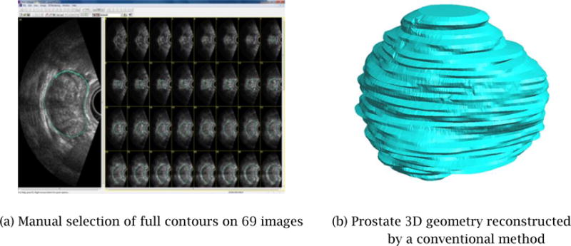
A prostate 3D geometry reconstructed from a set of manually selected full contours is not smooth and may not be watertight.
There have been several published methods on automated or semi-automated reconstruction of 3D prostate shapes [20, 21, 22, 23]. These methods typically create contours by using automated image processing and/or active contours – physically based curve models to create a contour that is of a specified level of smoothness. After a set of contours is specified, some of the methods fit a deformable 3D model to the set of contours to yield a watertight 3D prostate shape. In contrast to these conventional approaches which require a specification of full contours in the original 2D TRUS images, our new method presented in this paper allows the user to select the best cross-sectional directions and draw only clearly recognizable partial contours. The user can thus avoid time-consuming and inaccurate guesswork on where prostate contours are located. The proposed method also yields more accurate prostate shapes than conventional methods by avoiding the usage of noisy, incomprehensible portions of the TRUS image.
The 3D prostate shape reconstruction problem presented in this paper can be stated as follows:
Input
A 3D TRUS image of a prostate: a set of gray-scale 2D TRUS images arranged sequentially in 3D space, forming a volumetric image.
Output
A 3D surface model of the prostate as a 3D polygonal mesh.
Requirements
- Target accuracy: 2 mm for contour specification and smooth interpolation
- Processing time: five minutes in total
- Water-tightness of the output surface model
- Realistic and natural shape suitable for surgical planning and training applications
The rest of this paper is organized as follows. Section 2 presents the outline and the detail of the proposed two-step method. Section 3 shows the results of three experimental cases; the first validates the first step of the proposed method, the second validates the second step of the proposed method, and the third validates the effectiveness of the total process. Section 4 presents the conclusions and future work.
2 Proposed Computational Method for 3D Shape Reconstruction
The proposed method takes as input a 3D TRUS image and generates a 3D surface model of the prostate as a 3D polygonal mesh by using the two-step approach illustrated in Fig. 3: (1) the user specifies partial contours on cross-sectional images with arbitrary orientations, and (2) the system automatically deforms a template mesh to fit the partial contours.
Figure 3.
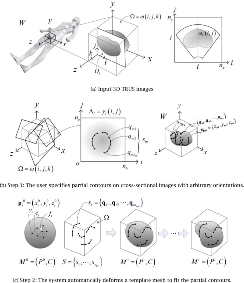
Proposed two-step approach to generating the 3D surface model of a prostate from a 3D TRUS image
Throughout the entire process, the position and orientation of the 3D TRUS images, cross-sectional images, partial contours, the initial template geometry, and the final 3D surface geometry are represented in the coordinate system attached to the patient’s body. This world coordinate system, denoted as W, is oriented as illustrated in Fig. 3(a), that is, the xy_-plane represents the traverse plane, the xz-plane the sagittal plane, and the yz-plane the coronal plane. A 3D TRUS image is a sequence of nk 2D images, Ok,k = 1,⋯,nk, that are parallel to the traverse plane. The transformation from the world coordinate system, W, to each 2D image coordinate system, W_Ok, is provided from the 3D TRUS imaging system. A 3D TRUS image is a volumetric image represented by a 3×3×3 matrix that stores a grayscale intensity of voxels: Ω = ω(i,j,k), i = 1,⋯,ni, j = 1,⋯,nj, k = 1,⋯,nk, where ni, nj, and nk are the number of voxels in the x, y and z directions respectively. The size of a voxel is defined by its length in the x, y, and z directions: Δ_x_, Δ_y_, and Δ_z_.
The input 3D TRUS image is processed in two steps. The first step, Step 1, is an interactive process where the user navigates through the 3D TRUS image by taking cross sections in arbitrary positions and orientations, freely adjusts the cross-sectional images’ contrast and intensity, and specifies partial or full contours of the prostate. As illustrated in Fig. 3(b), a set of cross-sectional images is denoted as Λ_l= γl_(i,j),i = 1,⋯,nh, j = 1,⋯,nv, l = 1,⋯,nl, where nh and nv are the number of pixels in the x and y directions respectively, and nl is the number of cross-sectional images. The coordinate transformation from the world coordinate to cross-sectional image coordinate, Λ_l_, is denoted as w_Λ_l. On each cross-sectional image, the user may specify multiple partial contours. All the partial contours are transformed to 3D line segments represented in the world coordinate system. This set of nm 3D contours is denoted as S={s1,⋯,snm} where each contour consists of a sequence of nmi 3D points, si=(qi1,⋯,qinmi),i=1,⋯,nmi.
The second step, Step 2, is an automated process where template geometry, represented by a polygonal mesh, is deformed to fit the user-specified contours. The mesh is represented as a pair, _M_0 =(_P_0,C), where _P_0 is a set of nv points in IR3,P0={p10,⋯,pnv0} and C is topological connectivity information that contains a set of nv vertices V={v1,⋯,vnv}, a set of ne edges E={e1,⋯,ene} and a set of nf faces F={f1,⋯,fnf}. Point pi0=(x,y,z) represents the geometric position of Vertex vi in the template mesh. In Step 2 the template mesh is deformed iteratively to fit the contours. The mesh after the _i_-th iteration is denoted as Mi =(Pi,C), where Pi represents the updated position of vertices. Note that the topological connectivity of the mesh, C, remains the same throughout Step 2. The template mesh will be progressively morphed into different meshes, _M_0 _→ M_1 →⋯→Mi →⋯→Mt, until it reaches the final mesh, Mt = (Pt, C).
The rest of Section 2 presents further details of Steps 1 and 2.
2.1 Step 1: Manual Specification of Partial Contours
With the GUI application developed for Step 1, the user can: (1) navigate through the 3D TRUS image freely by viewing cross-sectional images at arbitrary positions and orientations; (2) adjust the image intensity and contrast at any time of the navigation, and (3) specify partial or full contours on cross-sectional images. The system is built so that all the operations can be performed intuitively and easily using a standard PC mouse or digitizer.
As shown in Fig. 4(a), the system uses two graphics windows to display simultaneously: (1) a 3D view of a cross-sectional image and 3D contours; and, (2) a 2D view of a cross-sectional image and 2D contours. All the image processing calculations are performed by in-house software built with the VTK and ITK Toolkit [7, 8].
Figure 4.
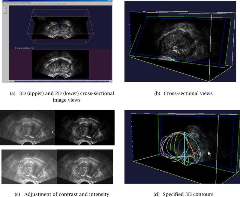
Developed GUI for Step 1 cross-sectional image navigation, adjustment of intensity and contrast, and specification of partial/full contours.
It should be noted that the proposed method would not work well if most of the partial contours are extracted from only a portion of the shape. This problem is avoided by giving the user real-time visual feedback as he/she adds each contour. The 3D view can be rotated freely so the user can avoid specifying contours only for a portion of the shape.
2.1.1 Real-time Cross-Sectional Image Display
Figure 4(b) shows examples of a cross-sectional image. The user controls the position and orientation of the cross-sectional plane by moving the mouse in both horizontal and vertical directions. The cross-sectional image is updated in real-time, with a refreshing rate of 5–10 frames per second – the actual refreshing rate depends upon the performance of the graphics card installed on the PC. This range of refreshing rate of a cross sectional image is sufficient for a stress-free interaction with a 3D TRUS image.
2.1.2 Image Intensity and Contrast Adjustment
The current GUI system allows the user to adjust the intensity and contrast of a cross-sectional image in real-time, by a combination of a keystroke and mouse movement (see Fig. 4(b)). The intensity and contrast adjustment is similar to the function that is available in commercial/non-commercial image processing software packages, such as Adobe Photoshop [9] and IrfanView [10]. It is our future plan to enhance the image processing capability of the system to include fairing and de-noising operations [11].
2.1.3 Specification of Partial/Full Contours
Figure 4(d) shows a set of partial contours specified by the user on 10–15 cross-sectional images. The users can display a 3D view of the partial contours anytime during Step 1 in order to decide if a sufficient number of contours has been specified or not.
2.2 Step 2: Automated Smooth Interpolation of Partial Contours
While the GUI and functionality design of Step 1 is relatively straightforward, the selection of the best mesh deformation method for Step 2 requires extensive benchmarking and comparison of multiple candidates.
The key requirements to consider in designing the computational method for Step 2 are:
- the method must interpolate a limited number of partial contours to form a natural prostate shape;
- the surface of the generated 3D prostate shape must be smooth and realistic;
- the computational cost for converging to the final shape must be low enough to complete in about a minute with a standard PC; and,
- the method must create a water-tight polygonal mesh with no self-intersections.
2.2.1 Template Polygonal Mesh
In order to select the type and appropriate level of detail of the initial template mesh, _M_0, we computational experiments using two types of polygonal meshes – tri mesh and conducted computational experiments using two types of polygonal meshes – tri mesh and quad mesh – of different mesh sizes. Several meshes were created for benchmarking with the number of mesh elements ranging from 200 to 2,000, examples of which are shown in Fig. 5. Figure 6 compares how a triangular-mesh template with 320 elements and a quadrilateral-mesh template with 384 elements each minimize the error between the final deformed mesh, Mt, and the correct 3D geometry of the prostate. In order to compare the performance of template polygonal meshes of different numbers of nodes and elements, we used one of the reconstructed 3D shapes as the true 3D shape. Note that this 3D shape can be any 3D prostate shape for the purpose of the comparison.
Figure 5.

Template polygonal models of the prostate
Figure 6.
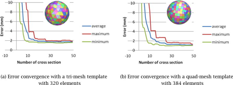
Error convergence with tri-mesh and quad-mesh templates. A quad-mesh template yields 30–40% smaller error compared with a tri-mesh template having a similar number of mesh elements.
The result of the computational experiment determined that:
- _M_0 of 300–400 elements would have the fewest possible number of mesh elements that yields 1.5 mm or less error (Fig. 6);
- A quad mesh yields a 30–40% more accurate result compared with a tri mesh having approximately the same number of elements.
Based on these observations, we chose to use the quad-mesh shown in Fig. 5(c) as the initial template mesh.
2.2.2 Comparison of Mesh-Smoothing Methods
To select the smoothing method that best satisfies the four requirements of Step 2, discussed at the beginning of Section 2.2, we implemented 17 mesh-smoothing schemes and compared the accuracy of each method. These smoothing schemes were: (1) Laplacian, (2) length-weighted Laplacian, (3) angle-weighted Laplacian, (4) area-weighted Laplacian, (5) curvature flow, (6) bi-harmonic Laplacian, (7) length-weighted bi-harmonic Laplacian, (8) angle-weighted bi-harmonic Laplacian, (9) area-weighted bi-harmonic Laplacian, (10) multi-layer Laplacian, (11) Gauss Laplacian, (12) single-layer Loop, (13) multi-layer Loop, (14) plane fitting, (15) quadratic surface fitting, (16) cubic surface fitting, and (17) V-spring. These methods are described in literatures [12–20].
The comparison of the mesh-smoothing methods was performed as follows. A pre-defined polygonal model of a prostate was designated as the ground-truth shape. We then created different sets of 3D contours by taking cross sections of different orientations including the directions parallel to the _xy_-plane, _yz_-plane and _zx_-plane of the 3D TRUS image coordinate frame, O. We used two sets of 3D contours, one with 13 cross-sectional images and the other with 25 cross-sectional images. For each of the 17 mesh-smoothing methods, therefore, we had six error numbers, each of which measured the average error between the ground-truth shape and the shape generated by deforming the template mesh to fit the input 3D contours. Although there are slight variations between two different input 3D contour sets, we could still see which method generally yields the smallest error. According to the results displayed in Fig. 7, we concluded that the V-Spring method [18, 19] performs the best, and hence it is our method of choice for mesh smoothing. It is not very surprising that V-Spring performs well for our application, as the method is designed to minimize curvature variation, and our target organ, the prostate, is a smooth round shape with no acute curvature change. Details of the V-Spring method are presented in the next section.
Figure 7.
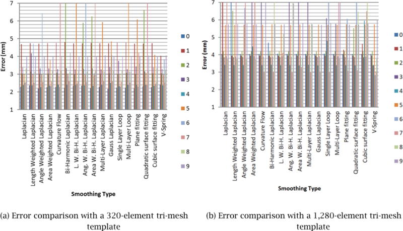
3D Error comparison with various smoothing schemes.
2.2.3 Proposed Mesh Smoothing Method – V-Spring
As concluded from the comparison study presented in Section 2.2.2, we chose to use the V-Spring method, originally proposed by Yamada et al. [18, 19] for generating a smooth polygonal mesh of the prostate. This section presents an overview of the V-Spring method and explains how it was adapted to generate a 3D prostate shape for the cryosurgical training application.
V-Spring is a computational method for generating a smooth polygonal surface by iteratively updating a mesh shape with two types of internal spring forces applied to vertices: (1) a spring force that acts in the normal direction to minimize the curvature variation, and (2) a spring force that acts in the tangential direction to optimize vertex distribution. For the first type of internal force, a spring is attached to each of the vertices, V={v1,⋯,vnv}, of the initial mesh _M_0. For a convex shape, these neighboring springs form a “V” shape, thus giving the name to the method. The spring length approximately represents the local curvature. During the iterative mesh deformation process, the springs work together to equalize their lengths to minimize the curvature variation of the surface, as illustrated in Fig. 8. Based on the spring model, in each deformation iteration the displacement of Vertex vi due to its neighboring vertex, vj, is calculated as followed (see [18, 19] for details):
| δa=1‖pj−pi‖[(pj−pi)⋅(ni+nj)1+(ni⋅nj)]ni, | (1) |
|---|
where pi and pj are the positions of Vertices vi and vj, respectively, and ni and nj are the unit normal vectors at Vertices vi and vj, respectively. The total normal displacement, Δai, of vi due to all of its neighboring vertices is then calculated as the vector sum of all the displacements:
where m is the number of neighboring vertices of Vertex vi.
Figure 8.
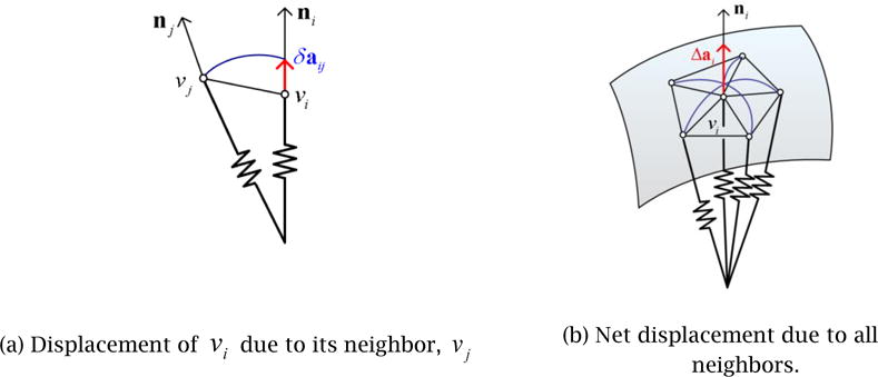
V-Spring uses a spring force that acts in the normal direction to minimize curvature variation.
In addition to the normal displacement, the V-Spring method also defines the second type of springs and internal forces to optimize the vertex distribution, as illustrated in Fig. 9. The process is a modified Laplacian smoothing process in which each vertex is connected to its neighboring vertices by a linear spring of zero neutral length. A vertex is moved toward the barycenter of its neighbors to maintain a uniform vertex distribution. The modification from the original Laplacian smoothing is to limit the motion of a vertex to the tangential direction. The tangential displacement due to one of the neighboring vertices is calculated as
| δbij=1m[pj−pi−[(pj−pi)⋅ni]ni], | (3) |
|---|
where m is the number of neighboring vertices. The total tangential displacement, Δbi, is then calculated as the vector sum of all the displacements:
Figure 9.
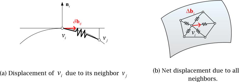
V-Spring uses a spring force that acts in the tangential direction to optimize vertex distribution.
While the above-mentioned two types of springs and internal forces make the final surface shape smooth, a third type of springs and external forces is used for fitting, or constraining, the final surface to approximate the set of partial contours, S={s1,⋯,snm}. Recall that each contour consists of a sequence of nmi 3D points,
| si=(qi1,⋯,qinmi),i=1,⋯,nmi | (4) |
|---|
Although the V-Spring method allows direct constraints by which the final surface interpolates exactly the set of contours points, this is not appropriate for our application because the user’s input of the partial contours in Step 1 is not exact and may be slightly contradictory. We thus adopt indirect constraints by which the final surface approximates the contour points but does not interpolate them. In this way, if the input contour points are contradictory, an average solution is created. The surface is fitted to the partial contours by defining springs that move the surface in the normal direction. The displacement of Vertex vi due to a spring that connects the vertex and one of the contour points, qjk, is calculated as:
| δcijk=kjk[(qjk−pi)⋅ni]ni, | (5) |
|---|
where kjk denotes a weight assigned to qjk and represents a weighted component of vector (q_jk_−pi) along the normal vector, ni. In each deformation iteration, these two displacements are combined to update the positions and normals of each vertex, morphing the initial mesh, _M_0, iteratively to the final mesh, Mt. The total displacement in the normal direction due to the external forces from all the contour points is then calculated as a weighted average:
| Δci=∑j=kn∑k=1nmiwjkδcijk∑j=kn∑k=1nmiwjk, | (6) |
|---|
where wjk are weights for averaging. In the current implementation, the weights are calculated as the inverse of the distance from Vertex vi to the foot of the perpendicular of contour point qjk onto the tangent plane (see Figure 10):
| wjk=[(qjk−pi)−[(qjk−pi)⋅ni]ni]−1. | (7) |
|---|
Figure 10.
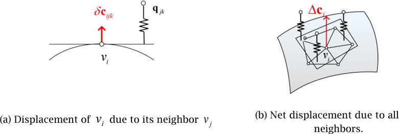
V-Spring uses spring forces for fitting, or constraining, the final surface to approximate the set of partial contours.
With the two internal spring forces combined with the external force, the total displacement of Vertex vi in each deformation iteration is defined as the sum of three displacements:
The iterative deformation morphs the initial template mesh, _M_0, into a sequence of meshes, _M_1,M2,M,⋯, until the change of the mesh’s shape becomes less than a given threshold. The behavior of the V-Spring model changes depending on the balance among the three types of springs. For more details, see [18, 19].
3 Validation of the Proposed Shape-Reconstruction Method
Three case studies were conducted to validate the proposed shape-reconstruction method. The goal of each case study was as follows:
- Case Study 1: to confirm the effectiveness of the interactive GUI system developed for Step 1 and the consistency of contour plotting across different users.
- Case Study 2: to measure the accuracy, convergence, and computational cost of the V-Spring-based deformable surface fitting process of Step 2.
- Case Study 3: to demonstrate the performance of the entire 3D shape reconstruction process consisting of Step 1 and Step 2.
3.1 Case Study 1: Interactive Contour Specification in Step 1
In Step 1, using the interactive GUI system, the user adjusts, navigates through, and visualizes the input TRUS image to specify partial contours. The goal of Case Study 1 was two-fold: (1) to confirm that the developed GUI system is easy-to-use and efficient enough to specify a set of 10 ~ 15 cross-sectional planes and 20 ~ 30 partial contours within several minutes, and (2) to measure the consistency of contour plotting across different users and confirm that contours can be specified consistently within 2 mm for mid to high quality image regions.
Experiments were conducted as follows. For each of four randomly selected cross-sectional images, five users were asked to specify a closed contour. As the input TRUS image was fairly noisy with many speckles and shadows, the users were forced to guess about certain regions in drawing contours. Figure 11 shows the color-coded contours specified by the five different users. It is observed that for some regions where the image is clearer, the user-specified contours are more consistent and the average deviation is within 1.5 mm. For other regions where the image is less clear, the user-specified contours are less consistent, and the average deviation exceeds 2 mm.
Figure 11.
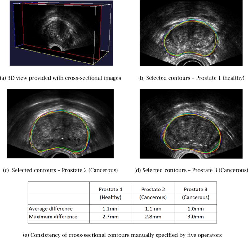
Manually specified contours deviate approximately 1 mm on average with a maximum deviation of 2.5–3.0 mm, if the user is asked to plot a complete contour.
The results of Case Study 1 suggest that the contour selection can be sufficiently accurate, (i.e., within 1.5mm) in order to be used in a computer-assisted cryosurgery trainer, when the user specifies partial contours in mid- to high-quality image regions only. The developed GUI system allows the user to do so with greater ease than the conventional image segmentation system. Specifying partial contours on each cross section takes 5 ~10 seconds including the selection of the cross-sectional plane. Specifying contours on a sufficient number (i.e., 10 ~ 15) of cross-sectional planes would take several minutes, but this time can be further reduced as the user becomes more proficient in using the GUI system.
3.2 Case Study 2: Validation of Surface Fitting in Step 2
The goal of Case Study 2 was to confirm that the accuracy, convergence, and computational cost of the proposed V-Spring-based deformable surface fitting meet the requirements.
In order to assess the accuracy of the shape reconstruction, a pre-defined polygonal model of the prostate was selected as the “ground truth” model. A pre-defined 3D shape was used here in order to measure the accuracy of the Step 2 process, even though the true shape is unknown in a real application scenario. A set of contours was generated by three schemes:
- Scheme 1: Full contours on multiple cross sections parallel to the _yz_-plane.
- Scheme 2: Full contours on cross-sectional planes with randomly generated positions and orientations.
- Scheme 3: Partial contours on cross-sectional planes with randomly generated positions and orientations.
The accuracy was measured by the error, or the average distance, between the ground-truth model and the deformed surface model. Figure 12 displays how the error diminishes as the number of contours increases for each of the three methods. For the input contours created by Schemes 1 and 2, the error converges after 15 ~ 25 contours, while the input contours created by Scheme 3 require 25 ~ 30 contours for a convergence. Note that the nature of user-specified contours in a real application is between that of Scheme 2 and Scheme 3. In Scheme 3, the error does not converge monotonically and exhibits a significant amount of fluctuation. This is because the random selection of partial contours on each cross sectional plane yields shapes with larger variations. It should also be noted that a set of partial contours generated by Scheme 3 yields less accurate results than a set of evenly distributed partial contours specified carefully by the user. Thus, the error resulting from Scheme 3 leads to the most conservative estimation of the accuracy of the proposed surface-fitting method.
Figure 12.
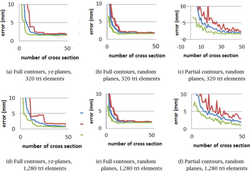
Error convergence with different types of input contours.
Figure 13 shows how the error is reduced as the number of partial contours created by Scheme 3 is increased. The result of this convergence study indicates that 20 ~ 30 partial contours are sufficient to bring the average error down to 1 mm and the maximum error down to 2 mm. This corresponds to 10 ~ 15 cross-sectional planes assuming that each cross-sectional plane contains two partial contours on average.
Figure 13.
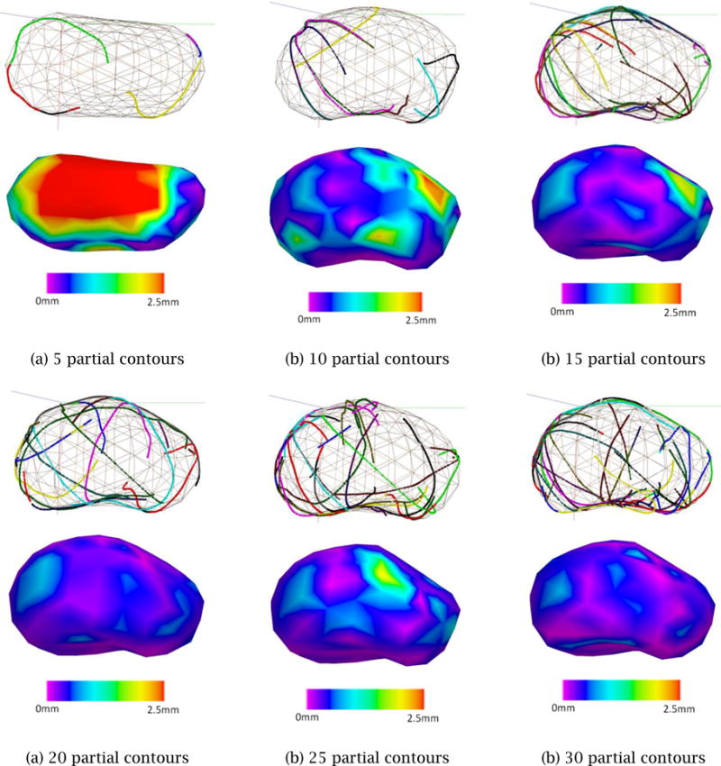
Shape convergence with multiple, randomly selected partial contours using Scheme 3
The computation time for the V-Spring-based surface fitting for 30 partial contours was approximately 2 seconds for a template with 320 tri elements and 5 seconds for a template with 1,280 tri elements. The computational time was measured on a standard Windows workstation with an Intel Core i5 2.44GHz CPU with 8GB of memory.
The result of Case Study 2 suggests that the accuracy, convergence characteristics, and computational cost of the proposed V-Spring-based method are suitable for the purpose of the Step 2 surface fitting.
3.3 Case Study 3: Validation of the Complete Process
The entire reconstruction process of Step 1 and Step 2 was performed to confirm that: (1) the surface of the generated 3D shape of a prostate was smooth and realistic; (2) the computational cost for converging to the final shape was low enough to finish within five minutes using a standard PC; and, (3) the method created a water-tight polygonal mesh with no self-intersections.
Figure 14 illustrates the entire Step 1 and Step 2 processes of the proposed shape reconstruction method. Figure 14(a) shows the Step 1 process of manual contour specification, and Fig. 14(b) shows a set of specified partial contours, which then become part of the input to the Step 2 deformable surface fitting. Figure 14(c) illustrates the convergence process of the V-Spring method. Figure 14(d) shows the final 3D shape of the prostate. Note that the user can choose the resolution of the final output model, and the system generates a finer mesh using a standard subdivision surface scheme. The final shape is a smooth, realistic, and watertight shape suitable for a computer-assisted cryosurgery training system.
Figure 14.
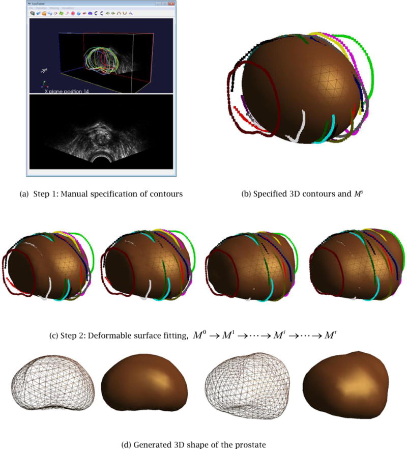
Case Study 3: the entire shape reconstruction process yields a smooth, realistic, and water-tight 3D shape of the prostate.
The same shape reconstruction process has been applied four times by different users to each of the five 3D TRUS images yielding the 20 3D prostate shapes shown in Figure 15. The figure shows for each trial: (1) specified 3D contours (left); (2) the generated 3D prostate shape superimposed on the specified 3D contours (middle); and (3) the generated 3D prostate shape (right).
Figure 15.
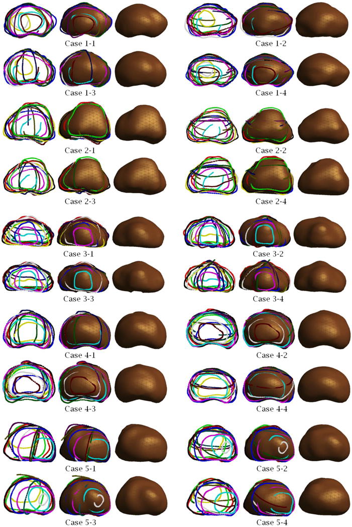
Examples of 3D prostate shapes created by the proposed shape reconstruction method.
To confirm the robustness and repeatability of the proposed 3D prostate shape reconstruction method, we measure seven error statistics including the Hausdorff distance, Dice’s coefficient, 25/50/75/95- percentile of the distance for the four reconstructed 3D prostate shapes for each TRUS image. Since the distance is directional, for each group of four 3D shapes, 12 sets of distance statistics are generated. The mean and the standard deviation of each set are summarized in Table 1. To further investigate the deviation between two shapes created from the same TRUS image, we select randomly one of the four reconstructed 3D shapes and measure the distances from the selected shape to the other three shapes. Figure 16 illustrates the distance distribution color-mapped on the 3D shape along with the distance histogram. The error statistics confirms the high level of robustness and repeatability of the proposed 3D shape reconstruction method.
Table 1.
Mean and standard deviation of the Hausdorff distance, Dice’s coefficient, 25 percentile, 50 percentile, 75 percentile and 95 percentile of the error distance.
| Statistics of error distance | Case 1 | Case 2 | Case 3 | Case 4 | Case 5 | |
|---|---|---|---|---|---|---|
| Hausdorff | Mean (mm) | 0.4484 | 0.9058 | 0.4719 | 0.5283 | 0.7665 |
| Standard deviation (mm) | 0.0486 | 0.1152 | 0.0850 | 0.0600 | 0.2085 | |
| Dice’s coefficient | Mean (mm) | 0.9544 | 0.9428 | 0.9493 | 0.9655 | 0.9441 |
| Standard deviation (mm) | 0.0085 | 0.0114 | 0.0108 | 0.0066 | 0.0171 | |
| 25 percentile | Mean (mm) | 0.0325 | 0.0491 | 0.0308 | 0.0264 | 0.0292 |
| Standard deviation (mm) | 0.0111 | 0.0145 | 0.0106 | 0.0092 | 0.0129 | |
| 50 percentile | Mean (mm) | 0.0720 | 0.1163 | 0.0638 | 0.0572 | 0.0693 |
| Standard deviation (mm) | 0.0205 | 0.0288 | 0.0177 | 0.0155 | 0.0258 | |
| 75 percentile | Mean (mm) | 0.1325 | 0.2340 | 0.1109 | 0.1061 | 0.1422 |
| Standard deviation (mm) | 0.0249 | 0.0514 | 0.0232 | 0.0219 | 0.0439 | |
| 95 percentile | Mean (mm) | 0.2425 | 0.4942 | 0.2142 | 0.2333 | 0.4001 |
| Standard deviation (mm) | 0.0279 | 0.1028 | 0.0386 | 0.0334 | 0.1447 |
Figure 16.
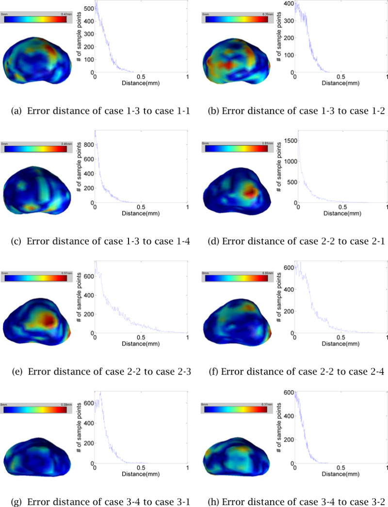
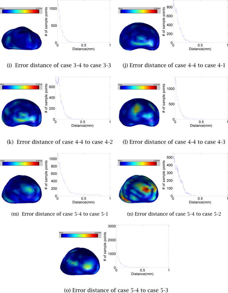
The error distances map and histogram of a process to the other process for each case
4 Summary and Conclusions
A 3D TRUS image-based shape reconstruction method for the prostate is proposed. Generated shapes are smooth, realistic, and water-tight, making the method suitable for a computerassisted trainer for prostate cryosurgery. Because the system lets the user adjust, navigate through, and visualize the TRUS images freely, the user can choose a set of cross-sectional images and specify partial contours of the prostate with a high level of confidence. The system then creates a complete prostate shape using deformable mesh smoothing. The entire 3D shape reconstruction process takes only several minutes, and the resulting shape is more realistic and accurate than a 3D shape created by a conventional method that uses an automated image segmentation technique.
As future work, we plan to automate the specification of partial contours in Step 1. Although the complete contour identification is challenging for low- to medium-quality TRUS images, we do not need to generate complete contours if we use the fully automated deformable mesh fitting scheme proposed in this paper – this will alleviate the difficulty of the automated contour specification. After adjusting the intensity and contrast and applying various noise-reduction filters automatically, the image processing method should be able to specify automatically the partial contours that can be identified with a high level of confidence, mimicking the Step 1 process performed by the user.
Acknowledgments
The authors would like to thank Dr. Aaron Fenster and his colleagues at the Robarts Research Institute of The University of Western Ontario, London, Ontario, Canada, for providing all the 3D TRUS images used in our research project.
This study was supported by Award Number R01CA134261 from the National Cancer Institute. The content is solely the responsibility of the authors and does not necessarily represent the official views of the National Cancer Institute or the National Institutes of Health. The development of the V-Spring method was supported by a CAREER Award from the National Science Foundation, a research grant from IBM, and a research grant from Honda R&D.
References
- 1.Rossi M, Tanaka D, Shimada K, Rabin Y. Computerized Planning of Prostate Cryosurgery Using Variable Cryoprobe Insertion Depth. Cryobiology. 2010;60(1):71–79. doi: 10.1016/j.cryobiol.2008.11.008. [DOI] [PMC free article] [PubMed] [Google Scholar]
- 2.Tanaka D, Shimada J, Rossi M, Rabin Y. Cryosurgery Planning Using Bubble Packing in 3D. Computer Methods in Biomechanical and Biomedical Engineering. 2008;11(2):113–121. doi: 10.1080/10255840701336653. [DOI] [PMC free article] [PubMed] [Google Scholar]
- 3.Developing a computerized training tool for cryosurgery. http://projectreporter.nih.gov/project_info_description.cfm?projectnumber=1R01CA134261-01A2.
- 4.Fenster A, Downey D, Cardinal N. Three Dimensional Ultrasound Imaging. Physics in Medicine and Biology. 2001;46(5):67–99. doi: 10.1088/0031-9155/46/5/201. [DOI] [PubMed] [Google Scholar]
- 5.Tong S, Downey D, Cardinal N, Fenster A. A three-dimensional ultrasound prostate imaging system. Ultrasound Med, Biol. 1996;22:735–746. doi: 10.1016/0301-5629(96)00079-8. [DOI] [PubMed] [Google Scholar]
- 6.3D Doctor. http://www.ablesw.com/3d-doctor/
- 7.The Visualization Toolkit. http://www.vtk.org.
- 8.ITK – Segmentation & Registration Toolkit. http://www.itk.org.
- 9.Adobe Photoshop. http://www.adobe.com/PhotoshopCS5.
- 10.IrfanView. http://www.irfanview.com.
- 11.Image Processing Toolbox for MATLAB & Simulink. http://www.mathworks.com/products/image.
- 12.Desbrun M, Meyer M, Schroder P, Barr A. Implicit Fairing of Irregular Meshes using Diffusion and Curvature Flow. SIGGRAPH. 1999;99:317–324. [Google Scholar]
- 13.Helenbrook BT. Mesh deformation using the biharmonic operator. Int J Numer Methods Eng. 2003;56:1007–1021. [Google Scholar]
- 14.Guskov I, Sweldens W, Schroder P. Multi-resolution Signal Processing for Meshes. SIGGRAPH. 1999;99:325–334. [Google Scholar]
- 15.Vieira M, Shimada K, Furuhata T. Smoothing of Noisy Laser Scanner Generated Meshes Using Polynomial Fitting and Neighborhood Erosion. Journal of Machanical Design. 2004;126:495–503. [Google Scholar]
- 16.Li Z, Ma L, Jin X, Zheng Z. A New Feature-preserving Mesh-smoothing Algorithm. Visual Comput. 2009;25:139–148. [Google Scholar]
- 17.Vieira M, Shimada K. Surface Mesh Segmentation and Smooth Surface Extraction through Region Growing. Computer-Aided Geometric Design. 2005;22(8):771–792. [Google Scholar]
- 18.Yamada A, Furuhata T, Shimada K, Hou K. A Discrete Spring model for Generating Fair Curves and Surfaces. PG 99: Proceedings of the 7th Pacific Conference on Computer Graphics and Applications. 1999 [Google Scholar]
- 19.Shimada K, Yamada A, Tomotake T, Hou K-H. US Patent US6,226,405. Method and Apparatus for Updating Node Position. issued 2001.
- 20.Ghanei A, Soltanian-Zadeh H, Ratkewicz A, Yin FF. A Three-Dimensional Deformable Model for Segmentation of Human Prostate from Ultrasound Images. Medical Physics. 2001;28:2147–53. doi: 10.1118/1.1388221. [DOI] [PubMed] [Google Scholar]
- 21.Hu N, Downey DB, Fenster A, Ladak HM. Prostate Surface Segmentation from 3D Ultrasound Images. Proceedings IEEE International Symposium on Biomedical Imaging USA; IEEE Computer Society Press; 2002. pp. 613–6. [Google Scholar]
- 22.Mahdavi S, Chng N, Spadinger I, Morris WJ, Salcudeana SE. Semi-Automatic Segmentation for Prostate Interventions. Medical Image Analysis. 2011;15:226–37. doi: 10.1016/j.media.2010.10.002. [DOI] [PMC free article] [PubMed] [Google Scholar]
- 23.Garnier C, Bellanger JJ, Wu K, Shu H, Costet N, Mathieu R, et al. Prostate segmentation in HIFU therapy. IEEE Trans Medical Imaging. 2011;30(3):792–803. doi: 10.1109/TMI.2010.2095465. [DOI] [PMC free article] [PubMed] [Google Scholar]