Interpreting predictive models with Skater: Unboxing model opacity (original) (raw)

Over the years, machine learning (ML) has come a long way, from its existence as experimental research in a purely academic setting to wide industry adoption as a means for automating solutions to real-world problems. But oftentimes, these algorithms are still perceived as alchemy because of the lack of understanding of the inner workings of these model (see Ali Rahimi, NIPS ’17). There is often a need to verify the reasoning of such ML systems to hold algorithms accountable for the decisions predicted. Researchers and practitioners are grappling with the ethics of relying on predictive models that might have unanticipated effects on human life, such as the algorithms evaluating eligibility for mortgage loans or powering self-driving cars (see Kate Crawford, NIPS ’17, “The Trouble with Bias”). Data Scientist Cathy O’Neil has recently written an entire book filled with examples of poor interpretability as a dire warning of the potential social carnage from misunderstood models—e.g., modeling bias in criminal sentencing or using dummy features with human bias while building financial models.

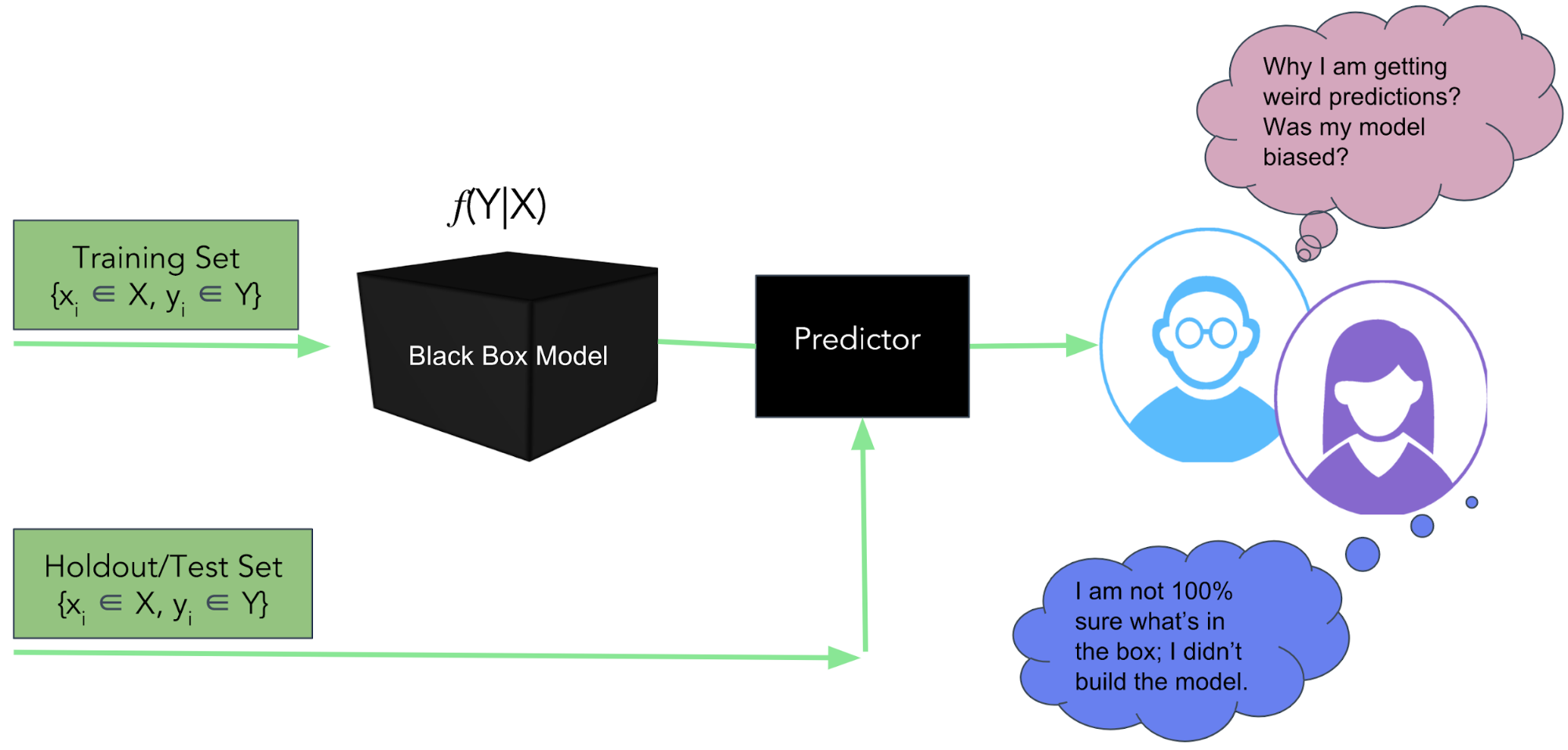
Figure 1. Traditional methods for interpreting predictive models are not enough. Image courtesy of Pramit Choudhary.

There is also a trade off in balancing a model’s interpretability and its performance. Practitioners often choose linear models over complex ones, compromising performance for interpretability, which might be fine for many use cases where the cost of an incorrect prediction is not high. But, in some scenarios, such as credit scoring or the judicial system, models have to be both highly accurate and understandable. In fact, the ability to account for the fairness and transparency of these predictive models has been mandated for legal compliance.

Learn faster. Dig deeper. See farther.

At DataScience.com, where I’m a lead data scientist, we feel passionately about the ability of practitioners to use models to ensure safety, non-discrimination, and transparency. We recognize the need for human interpretability, and we recently open sourced a Python framework called Skater as an initial step to enable interpretability for researchers and applied practitioners in the field of data science.

Model evaluation is a complex problem, so I will segment this discussion into two parts. In this first piece, I will dive into model interpretation as a theoretical concept and provide a high-level overview of Skater. In the second part, I will share a more detailed explanation on the algorithms Skater currently supports, as well as the library’s feature roadmap.

What is model interpretation?

The concept of model interpretability in the field of machine learning is still new, largely subjective, and, at times, controversial (see Yann LeCun’s response to Ali Rahimi’s talk). Model interpretation is the ability to explain and validate the decisions of a predictive model to enable fairness, accountability, and transparency in the algorithmic decision-making (for a more detailed explanation on the definition of transparency in machine learning, see “Challenges of Transparency” by Adrian Weller). Or, to state it formally, model interpretation can be defined as the ability to better understand the decision policies of a machine-learned response function to explain the relationship between independent (input) and dependent (target) variables, preferably in a human interpretable way.

Ideally, you should be able to query the model to understand the what, why, and how of its algorithmic decisions

• What information can the model provide to avoid prediction errors? You should be able to query and understand latent variable interactions in order to evaluate and understand, in a timely manner, what features are driving predictions. This will ensure the fairness of the model.
• Why did the model behave in a certain way? You should be able to identify and validate the relevant variables driving the model’s outputs. Doing so will allow you to trust in the reliability of the predictive system, even in unforeseen circumstances. This diagnosis will ensure accountability and safety of the model.
• How can we trust the predictions made by the model? You should be able to validate any given data point to demonstrate to business stakeholders and peers that the model works as expected. This will ensure transparency of the model.

Existing techniques capturing model interpretation

The idea of model interpretation is to achieve a better understanding of the mathematical model—which most likely could be achieved by developing a better understanding of the features contributing to the model. This form of understanding could possibly be enabled using popular data exploration and visualization approaches, like hierarchical clustering and dimensionality reduction techniques. Further evaluation and validation of models could be enabled using algorithms for model comparison for classification and regression using model specific scorers—AUC-ROC (area under the receiver operating curve) and MAE (mean absolute error). Let’s quickly touch on a few of those.

Exploratory data analysis and visualization

Exploratory data analysis can give one a better understanding of your data, in turn providing the expertise necessary to build a better predictive model. During the model-building process, achieving interpretability could mean exploring the data set in order to visualize and understand its “meaningful” internal structure and extract intuitive features with strong signals in a human interpretable way. This might become even more useful for unsupervised learning problems. Let’s go over a few popular data exploration techniques that could fall into the model interpretation category.

• Clustering: Hierarchical Clustering
• Dimensionality reduction: Principal component analysis (PCA) (see Figure 2)
• Variational autoencoders: An automated generative approach using variational autoencoders (VAE)
• Manifold Learning: t-Distributed Stochastic Neighbor Embedding (t-SNE) (see Figure 3)

In this article, we will focus on model interpretation in regard to supervised learning problems.

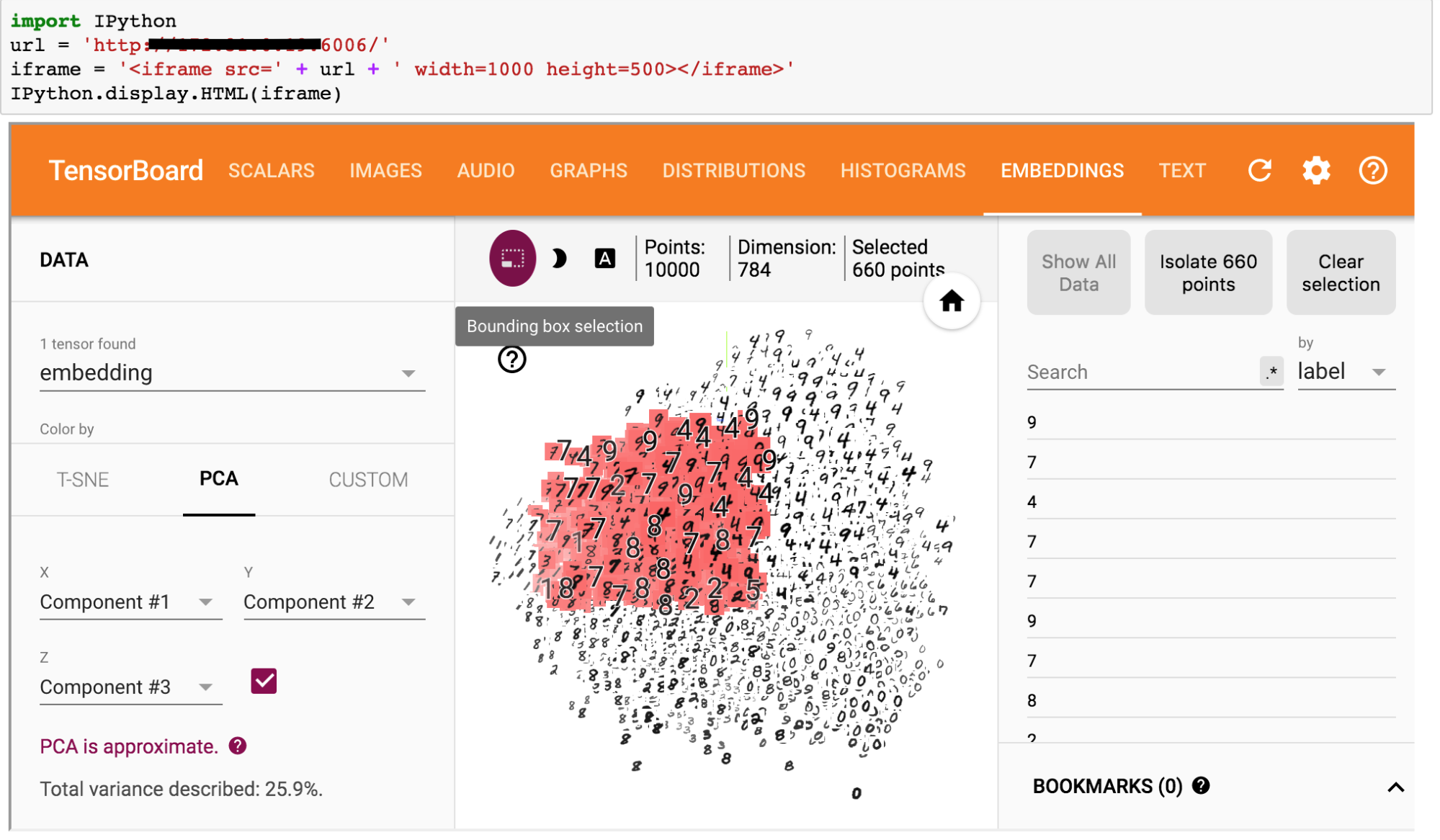
Figure 2. Interpreting high-dimensional MNIST data by visualizing in 3D using PCA for building domain knowledge using TensorFlow. Image courtesy of Pramit Choudhary and the Datascience.com team.

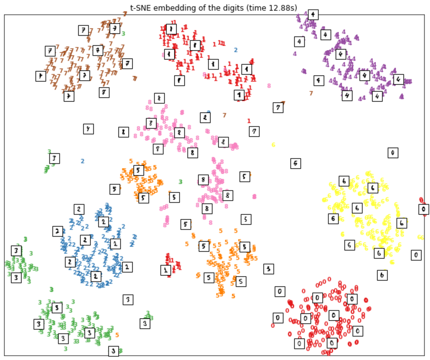
Figure 3. Visualizing MNIST data using t-SNE using sklearn. Image courtesy of Pramit Choudhary and the Datascience.com team.

B. model comparison and performance evaluation

In addition to data exploration techniques, model interpretation in a naive form could possibly be achieved using model evaluation techniques. Analysts and data scientists can possibly use model comparison and evaluation methods to assess the accuracy of the models. For example, with cross validation and evaluation metrics for classification and regression, you can measure the performance of a predictive model. You can optimize on the hyperparameters of the model balancing between bias and variance (see “Understanding the Bias-Variance Tradeoff“).

• Classification: for example, F1-scores, AUC-ROC, brier-score, etc. Consider Figure 3, which shows how AUC-ROC can help measure the model performance on a multi-class problem on the popular iris data set. ROC AUC is a widely popular metric that helps in balancing between true positive rate (TPR) and false positive rate (FPR). It’s pretty robust in handling class imbalances as well. As shown in Figure 3, a ROC AUC (class-2) of 86% means that the probability of the trained classifier assigning a higher score to a positive example (belonging to class-2) than to a negative example (not belonging to class-2) is about 86%. Such aggregated performance metric might be helpful in articulating the global performance of a model. However, it fails to give detailed information on the reasons for misclassification if an error occurs—why did an example belonging to Class 0 get classified as Class 2 and an example belonging to Class 2 get classified as Class 1? Keep in mind, each misclassification may have a varying potential business impact.
• Regression: for example, r-squared score (coefficient of determination), mean squared error, etc.

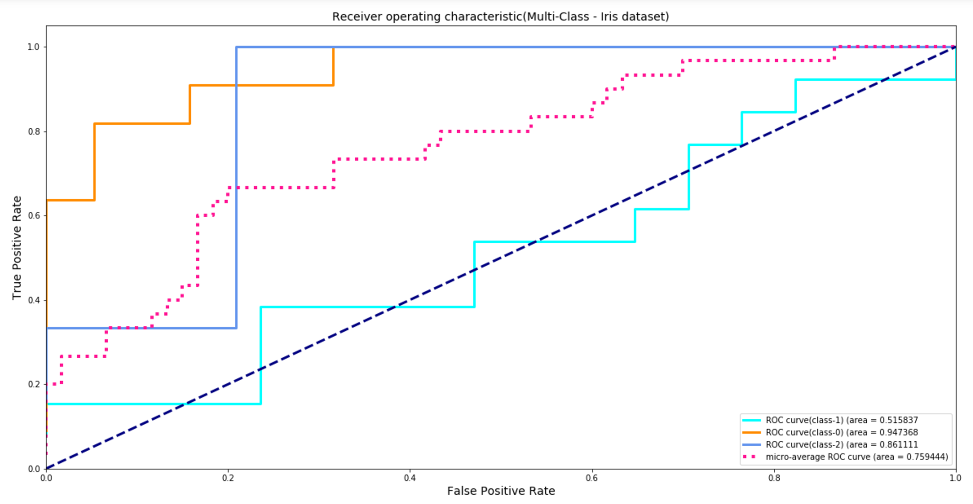
Figure 4. Measuring model performance by computing the area under the receiver operating characteristic curve (ROC curve) on the Iris data set, using sklearn for a multi-class problem. Image courtesy of Pramit Choudhary and the Datascience.com team.

Why the motivation for better model interpretation?

The above mentioned data exploration and point estimates computed using evaluation techniques might be sufficient in measuring the overall performance of a sample data set if the predictive model’s objective function aligns (the loss function one is trying to optimize) with the business metric (the one closely tied to your real-world goal), and the data set used for training is stationary. However, in real-world scenarios, that is rarely the case, and capturing model performance using point estimates is not sufficient. For example, an intrusion detection system (IDS), a cyber-security application, is prone to evasion attacks where an attacker may use adversarial inputs to beat the secure system (note: adversarial inputs are examples that are intentionally engineered by an attacker to trick the machine learning model to make false predictions). The model’s objective function in such cases may act as a weak surrogate to the real-world objectives. A better interpretation might be needed to identify the blind spots in the algorithms to build a secure and safe model by fixing the training data set prone to adversarial attacks (for further reading, see Moosavi-Dezfooli, et al., 2016, DeepFool and Goodfellow, et al., 2015, Explaining and harnessing adversarial examples).

Moreover, a model’s performance plateaus over time when trained on a static data set (not accounting for the variability in the new data). For example, the existing feature space may have changed after a model is operationalized in the wild or new information gets added into the training data set, introducing new unobserved associations, meaning that simply re-training a model will not be sufficient to improve the model’s prediction. Better forms of interpretations are needed to effectively debug the model to understand the algorithm behavior or to incorporate the new associations and interactions in the data set.

There might also be a use case where the model’s prediction natively is correct—where the model’s prediction is as expected—but it ethically fails to justify its decision in a social setting because of data biasedness (e.g., “Just because I like Kurosawa does not mean I want to watch 3 Ninjas”). At this point in time, a more rigorous and transparent diagnosis of the inner working of the algorithm might be needed to build a more effective model.

Even if one disagrees with all the above mentioned reasons as motivating factors for better interpretability needs, the traditional forms of model evaluation need a sound theoretical understanding of the algorithms or properties of statistical testing. It might be difficult for non-experts to grasp such details about the algorithm, often resulting in the failure of data-driven initiatives. A human interpretable interpretation(HII) of the model’s decision policies may provide insightful information that could easily be shared among peers (analysts, managers, data scientists, data engineers).

Using such forms of explanations, which could be explained based on inputs and outputs, might help facilitate better communication and collaboration, enabling businesses to make more confident decisions (e.g., risk assessment/audit risk analysis in financial institutions). To reiterate, we define model interpretation as being able to account for fairness (unbiasedness/non-discriminative), accountability (reliable results), and transparency (being able to query and validate predictive decisions) of a predictive model—currently in regard to supervised learning problems.

Dichotomy between Performance and Interpretability

There seems to be a fundamental trade-off between performance and algorithm interpretability. Practitioners often settle with easier interpretable models—simple linear, logistic regression, decision trees—because they are much easier to validate and explain. One is able to trust a model if one can understand its inner working or its decision policies. But, as one is trying to apply these predictive models to solve real-world problems with access to high-dimensional heterogeneous complex data sets—automating the process of credit applications, detecting fraud, or predicting lifetime value of a customer—interpretable models often fall short in terms of performance. As practitioners try to improve the performance (i.e., accuracy) of the model using more complex algorithms, they struggle to strike a balance between performance and interpretability.

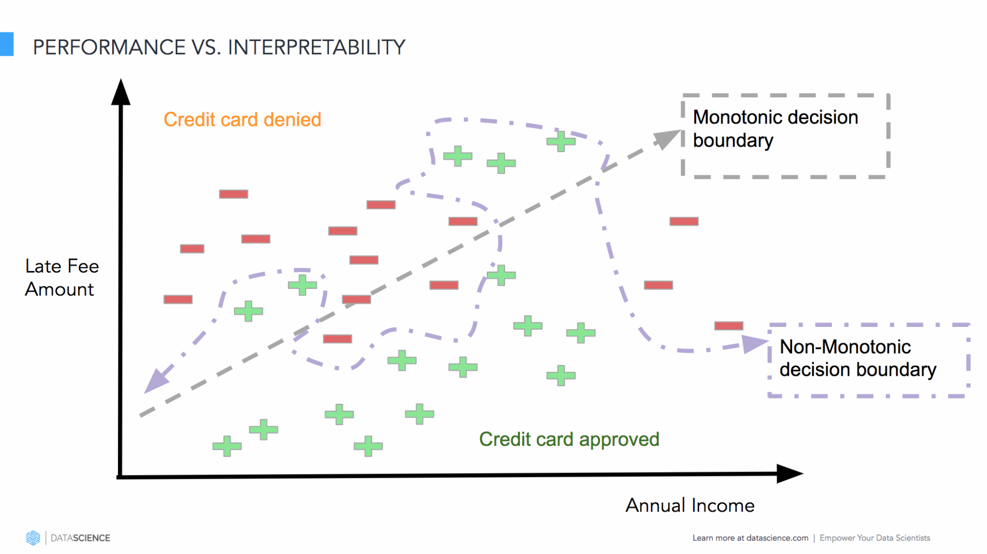
Figure 5. Model performance versus interpretability. Image courtesy of Pramit Choudhary and the Datascience.com team.

Let’s look at the problem of balancing performance and interpretability with an example. Consider the above Figure 5. Let’s assume one is building a model to predict the loan approval for a certain group of customers. Linear models (e.g., linear classifiers like logistic regression with log-loss or ordinary least square (OLS) for regression) are simpler to interpret because the relationship between the input variables and the model’s output could be quantified in magnitude and direction using the model’s coefficient weights. This line of thought works fine if the decision boundary is monotonically increasing or decreasing. However, this is rarely the case with real-world data. Hence, the perplexity in balancing between the model’s performance and interpretability.

In order to capture the non-monotonic relationship between the independent variable and the model’s response function, one generally has to make use of more complex models: ensembles, a random forest with a large number of decision trees, or a neural network with multiple hidden layers. The complexity increases further with text (Explaining Predictions of Non-Linear Classifiers in NLP using layer-wise relevance propagation (LRP)), computer vision (Ning et.al, NIPS’17, Relating Input Concepts to Convolutional Neural Network Decisions), and speech-based models with the need for human interpretability. For example, understanding of language-based models still remains a tough problem because of the ambiguity and uncertainty on the usage of similar words. Enabling human interpretability to understand such ambiguity in language models is useful in building use-case specific rules to understand, verify, and improve a model’s decision.

Introducing Skater

At Datascience.com, we have experienced interpretability challenges ourselves across different analytical use cases and projects, and understand the need for better model interpretation—preferably human interpretable interpretation (HII) expressed as inputs variables and model outputs (easily understood by non-experts). I specifically remember a project where we were building an ML model for summarizing consumer reviews. We wanted to capture the consumer sentiments (as positive or negative) as well as the specific reasons for each sentiment. Being time constrained, we thought it might be worth using an off-the-shelf model for sentiment analysis. We looked into many ML marketplace offerings, but we couldn’t decide on one to use because of trust issues and felt the need for better ways to interpret, verify, and validate models.

As we looked around, we couldn’t find a mature open source library that consistently enabled global (on the basis of a complete data set) and local (on the basis of an individual prediction) interpretation, so we developed a library from the ground up called Skater (see Figure 6).

Skater is a Python library designed with the goal to demystify the inner workings of any type of predictive model that is language and framework agnostic. Currently, it supports algorithms to enable interpretability with regard to supervised learning problems.

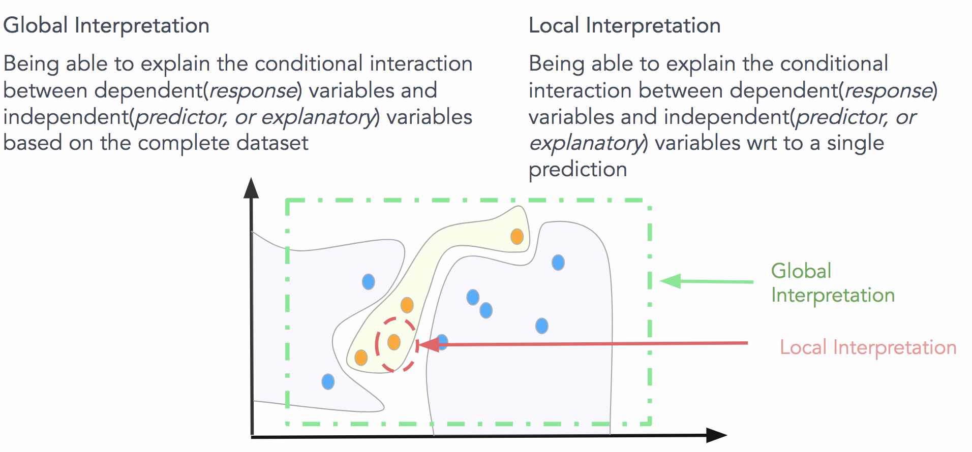
Figure 6. Summarizing global and local interpretation. Image courtesy of Pramit Choudhary and the Datascience.com team.

The interpretation algorithms currently supported are post-hoc in nature. As in, while Skater provides a post-hoc mechanism to evaluate and verify the inner workings of the predictive models based on independent (input) and dependent (target) variables, it does not support ways to build interpretable models (e.g., Rule Ensembles, Friedman, Bayesian Rule List).

This approach helps us to apply interpretability to machine learning systems depending on the analytical use cases—post-hoc operation could be expensive, and extensive interpretability may not be needed all the time. The library has embraced object-oriented and functional programming paradigms as deemed necessary to provide scalability and concurrency while keeping code brevity in mind. A high-level overview of such an interpretable system is shown in Figure 7.

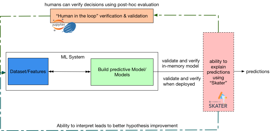
Figure 7. An interpretable ML system using Skater enabling humans to optimize generalization errors for better and more confident predictions. Image courtesy of Pramit Choudhary and the Datascience.com team.

Using Skater for model interpretation

Note: the complete code for the inline examples are added as reference links to the figures below.

With Skater one can:

• Evaluate the behavior of a model on a complete data set or on a single prediction: Skater allows model interpretation both globally and locally by leveraging and improving upon a combination of existing techniques. For global explanations, Skater currently makes use of model-agnostic variable importance and partial dependence plots to judge the bias of a model and understand its general behavior. To validate a model’s decision policies for a single prediction, the library embraces a novel technique called local interpretable model agnostic explanation (LIME), which uses local surrogate models to assess performance (here are more details on LIME). Other algorithms are currently under development.

from skater.core.explanations import Interpretation from skater.model import InMemoryModel ... eclf = VotingClassifier ( estimators = [( 'lr' , clf1 ), ( 'rf' , clf2 ), ( 'gnb' , clf3 )], voting = 'soft' ) ... models = { 'lr' : clf1 , 'rf' : clf2 , 'gnb' : clf3 , 'ensemble' : eclf } interpreter = Interpretation ( X_test , feature_names = data . feature_names ) Global interpretation with model agnostic feature importance for model_key in models : pyint_model = InMemoryModel ( models [ model_key ] . predict_proba , examples = X_test ) ax = ax_dict [ model_key ] interpreter . feature_importance . plot_feature_importance ( pyint_model , ascending = False , ax = ax ) ax . set_title ( model_key )

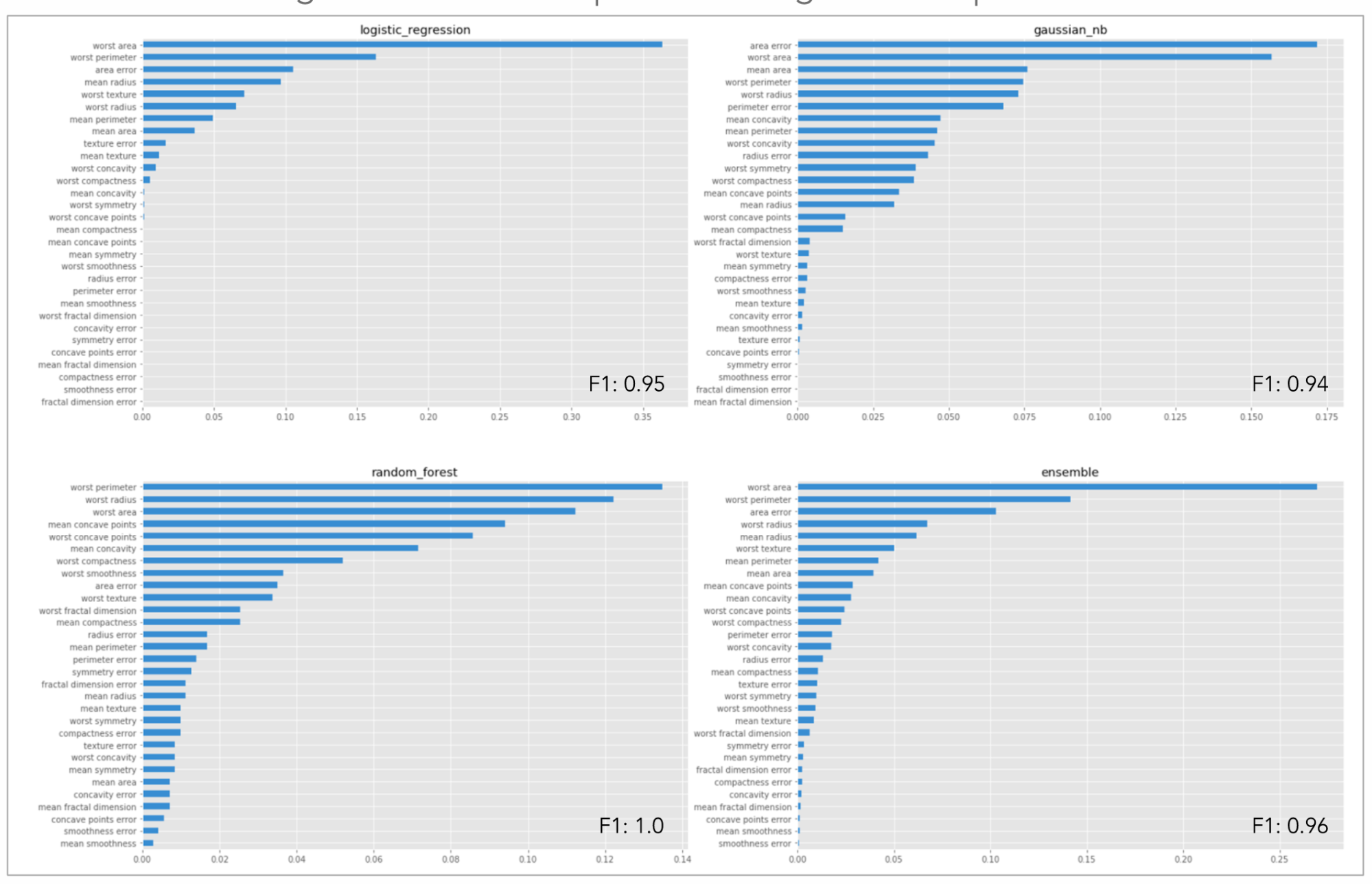
Figure 8. Model comparison using Skater between different types of supervised predictive models. Here, model agnostic feature importance is used to compare different forms of models with similar F1 scores. One can see different model types rank features differently based on the model’s assumption about the predictor, response variable and their relationship. This form of comparison allows experts and non-experts in the field of ML to evaluate selected feature relevance consistently. Image courtesy of Pramit Choudhary and the Datascience.com team.

• Identify latent variable interactions and build domain knowledge: Practitioners can use Skater to discover hidden feature interactions—for example, how a credit risk model uses a bank customer’s credit history, checking account status, or number of existing credit lines to approve or deny his or her application for a credit card, and then uses that information to inform future analyses.

# Global Interpretation with model agnostic partial dependence plot def understanding_interaction (): pyint_model = InMemoryModel ( eclf . predict_proba , examples = X_test , target_names = data . target_names ) # ['worst area', 'mean perimeter'] --> list(feature_selection.value) interpreter . partial_dependence . plot_partial_dependence ( list ( feature_selection . value ), Pyint_model , grid_resolution = grid_resolution . value , with_variance = True ) # Lets understand interaction using 2-way interaction using the same covariates # feature_selection.value --> ('worst area', 'mean perimeter') axes_list = interpreter . partial_dependence . plot_partial_dependence ([ feature_selection . value ], Pyint_model , grid_resolution = grid_resolution . value , with_variance = True )

Figure 9. Discover hidden feature interactions using one-way and two-way interaction on a breast cancer data set. Image courtesy of Pramit Choudhary and the Datascience.com team.

# Model agnostic local interpretation using LIME from skater.core.local_interpretation.lime.lime_tabular import LimeTabularExplainer ... exp = LimeTabularExplainer ( X_train , feature_names = data . feature_names , discretize_continuous = False , class_names = [ 'p(No Cancer)' , 'p(Cancer)' ]) exp . explain_instance ( X_train [ 52 ], models [ 'ensemble' ] . predict_proba ) . show_in_notebook ()

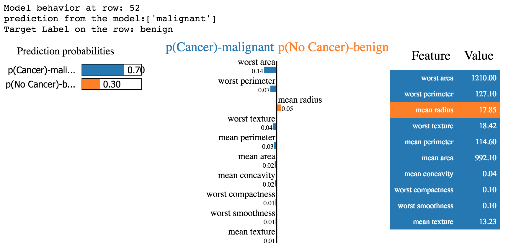
Figure 10. Understand feature relevance for a single prediction using a linear surrogate model via LIME. Image courtesy of Pramit Choudhary and the Datascience.com team.

• Measure how a model’s performance changes once it is deployed in a production environment: Skater enables consistency in the ability to interpret predictive models when in-memory as well as when operationalized, giving practitioners the opportunity to measure how feature interactions change across different model versions (See Figure 11). Such form of interpretation is also useful for enabling trust when using off-the-shelf predictive models from an ML marketplace—e.g., algorithmia. For example, in Figure 12 and Figure 13, an off-the shelf sentiment analysis model from indico.io and algorithmia are compared and evaluated side by side using Skater on an IMDB review on House of Cards. Both models predict a positive sentiment (1 is positive, 0 is negative). However, the one built by indico.io is considering stop words such as “is,” “that,” and “of,” which probably should have been ignored. Hence, even though indico.io returns a positive sentiment with a higher probability compared to algorithmia, one may decide to use the latter.

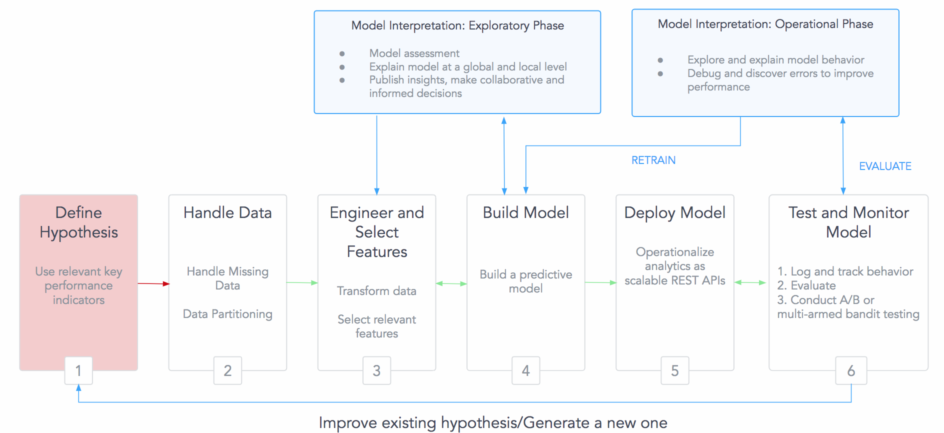
Figure 11. Highlighting need for interpretation for in-memory (model is not operationalized) and deployed model (model is operationalized). Better ways to interpret features might lead to better feature engineering and selection. Image source: image designed with help from Juhi Sodani and the Datascience.com team.

# Using Skater to verify third-party ML marketplace models from skater.model import DeployedModel from skater.core.local_interpretation.lime.lime_text import LimeTextExplainer ... #an example document test_documents = [ "Today its extremely cold, but I like it" ] #the API address algorithmia_uri = "https://api.algorithmia.com/v1/algo/nlp/SentimentAnalysis/1.0.3" ... dep_model = DeployedModel ( algorithmia_uri , algorithmia_input_formatter , algorithmia_output_formatter , request_kwargs = kwargs ) ... l = LimeTextExplainer () print ( "Explain the prediction, for the document: \n " ) print ( test_documents [ 0 ]) l . explain_instance ( test_documents [ 0 ] , dep_model , num_samples = 500 ) . show_in_notebook ()

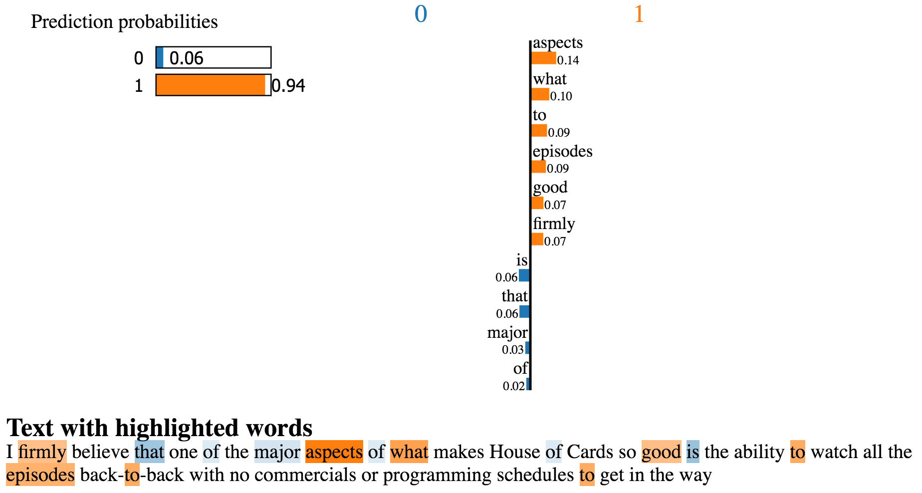
Figure 12. Enabling interpretability in using off-the-shelf models, pre-trained deployed model—indico.io. Image courtesy of Pramit Choudhary and the Datascience.com team.

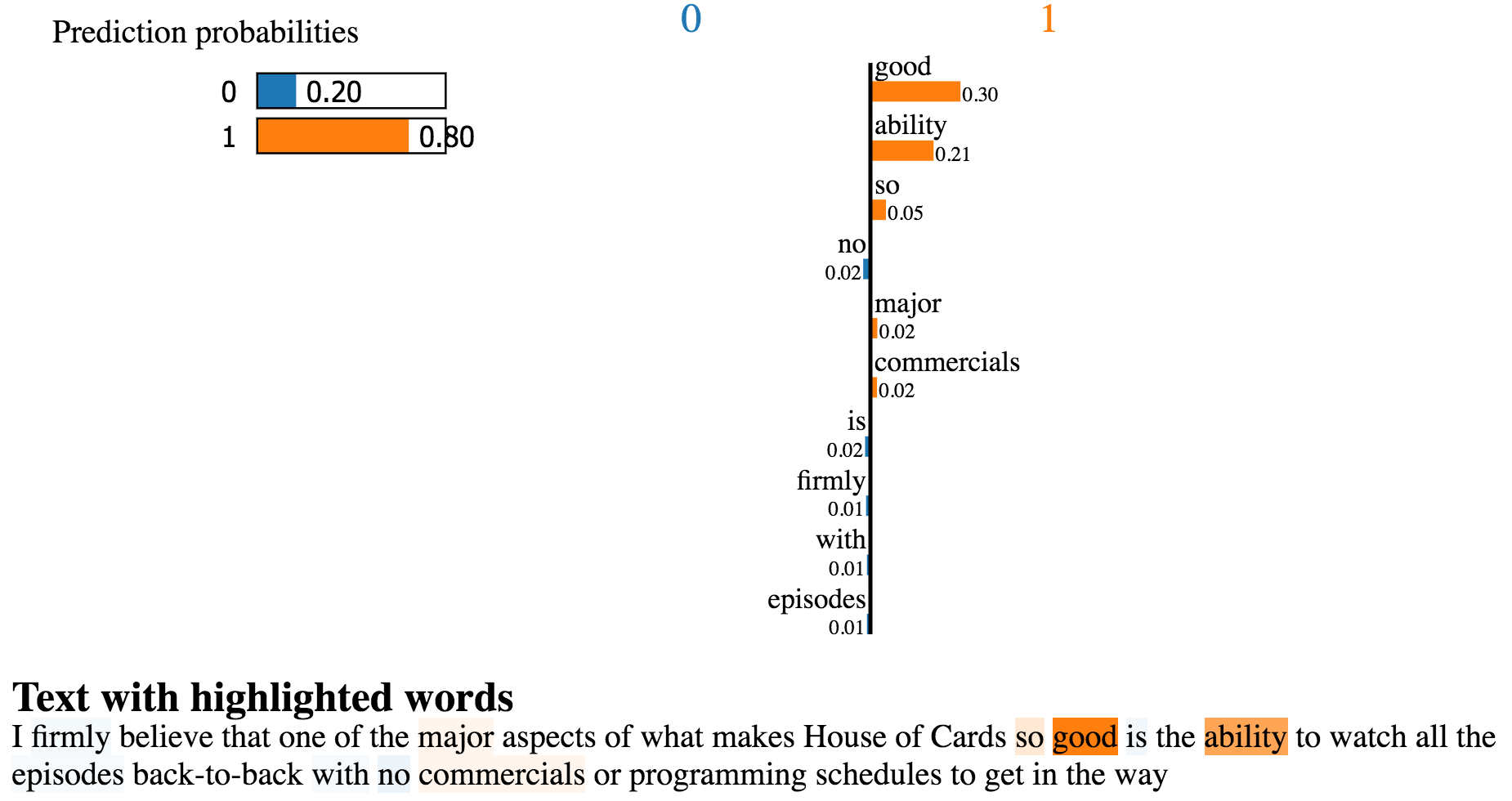
Figure 13. Enabling interpretability in using off-the-shelf models, pre-trained deployed model—algorithmia. Image courtesy of Pramit Choudhary and the Datascience.com team.

Conclusion

In today’s predictive modeling ecosystem, having means to interpret and justify the explanations of algorithmic decision policies in order to provide transparency will pay an important role. Having access to interpretable explanations might lead to the successful adoption of more sophisticated algorithms, especially in industries with regulatory needs. With the initial release of Skater, we are taking a step toward enabling fairness, accountability, and transparency of the decision policies of these predictive models for experts and non-experts in the field of machine learning. If you want to look at more examples of adopting Skater’s model interpretation capabilities in real-world examples, you can check out the book Practical Machine Learning with Python.

In the second part of this series, we will take a deeper dive into the understanding of the algorithms that Skater currently supports and its future road map for better model interpretation.

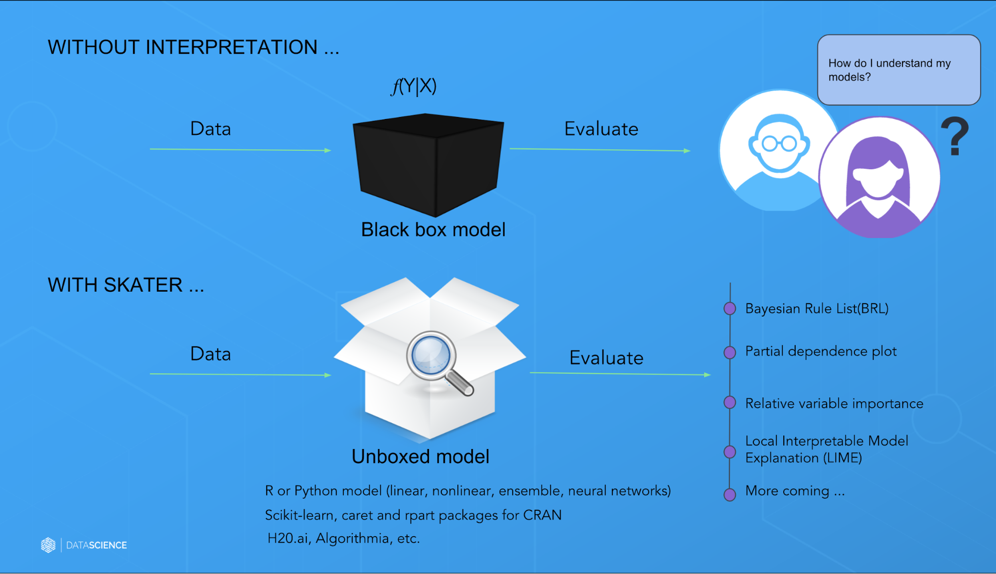
Figure 14. Summarizing Skater. Image courtesy of Pramit Choudhary and the Datascience.com team.

For more information, check out resources and tools, examples, or the gitter channel.