How to count unique values In Excel – 5 easy methods (original) (raw)
You can trust PC Guide: Our team of experts use a combination of independent consumer research, in-depth testing where appropriate - which will be flagged as such, and market analysis when recommending products, software and services. Find out how we test here.
If you want to learn how to count unique values in Excel, you’ve come to the right place.
Any kind of spreadsheet will contain both unique and distinct values. Unique values only appear once in a list, while distinct values are all the values that appear within a list. So, for example, if you had a list of numbers containing the values ‘1, 4, 7, 5, 7, 4’, then the unique values would be ‘1 and 5’ while the distinct values would be ‘1, 4, 7, and 5.’
AMD Ryzen 7 9800X3D returns to Amazon
AMD's Ryzen 7 9800X3D is finally back in stock on Amazon.US. Remember, use the "other sellers" button to ensure you get the best price through Amazon.
Prices correct as of November 14th, 2024.
When working in Excel, there may be occasions where you will need to identify how many unique values are contained within a list. So, to help you efficiently sort through the data, we put together this guide with 5 easy methods to teach you how to count unique values in Excel using various functions.
How to find out unique values from a dataset in Excel
Scenario on hand: We have a dataset with customer names who availed services at a beauty salon.
What we want to accomplish: Explore how to return values that are unique or distinct in the dataset using the following ways:
- Counting unique values with COUNTIF
- Counting unique text and numeric values
- Using the UNIQUE function
- Using the Advanced Filter option
- Using the filter for unique values
Counting unique values with COUNTIF
COUNTIF is a function in Excel that allows you to count values with a defined condition. Here are the steps to follow to use this method to count unique values in your dataset:
Step 1: Prepare the dataset
The first step is to prepare the dataset for the function. This formula returns the number of values that occur only once in the table. So, if you have data scattered across different sheets, consolidate it into one table.
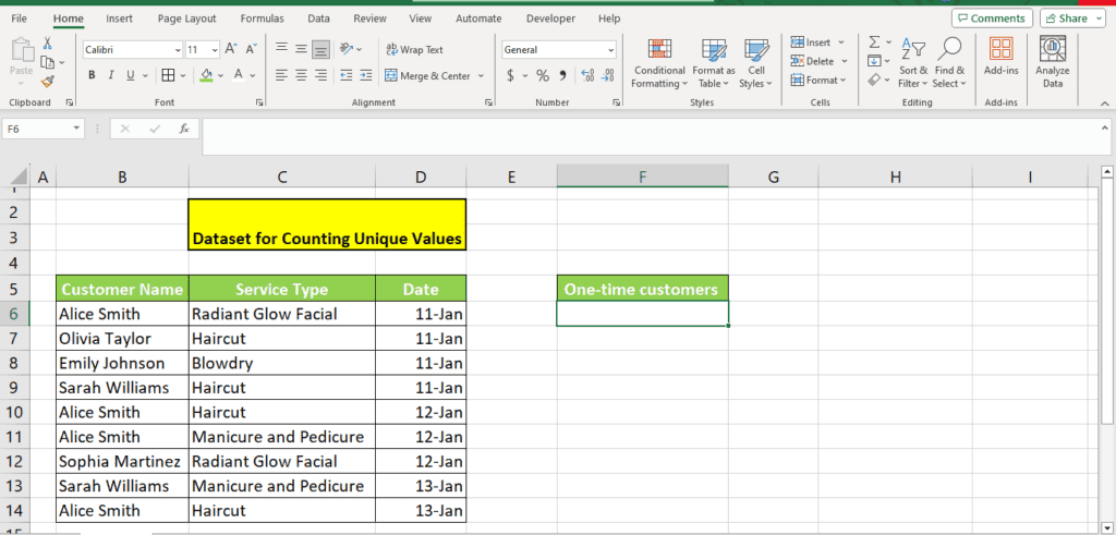
For our demonstration, we have a dataset with customer names and dates on which they availed services at a beauty salon:
Step 2: Enter the formula
In the cell where you want to get the number of unique values, type this COUNTIF formula:
=SUM(IF(COUNTIF({Column array, Column array})=1,1,0))
For our dataset, the formula looks like this:
=SUM(IF(COUNTIF(B6:B14,B6:B14)=1,1,0))
Here’s what this formula returns:
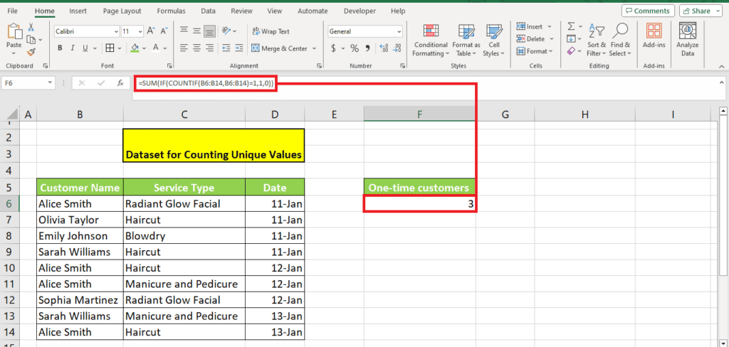
Note that this formula only gives us the count of the dataset’s unique values, not the unique ones. It also doesn’t differentiate between numeric and text values.
In the following method, we enter a formula that finds the number of unique text values and unique numeric values in the list.
Counting unique text and numeric values
This method lets you count the unique text and numeric values separately.
Step 1: Counting unique text values
You can add another function to the formula we used in the first method to search for a specific kind of unique value.
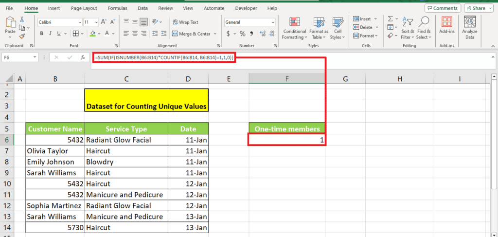
Let’s suppose that our dataset has two months of data. Suppose that we include numbers in place of customer names for those who have a membership card.
We want to ask whether customers with a membership card have availed beauty salon services once in two months to send them a special discount.
To search for these unique numerical values, here’s the altered formula we use:
=SUM(IF(ISNUMBER(data)*COUNTIF(data, data)=1,1,0))
For our dataset, we enter this formula:
=SUM(IF(ISNUMBER(B6:B14)*COUNTIF(B6:B14, B6:B14)=1,1,0))
Here’s what we get:
Step 2: Counting unique text values
Let’s try the text formula for getting the number of unique text values in our list:
=SUM(IF(ISTEXT(data)*COUNTIF(data, data)=1,1,0))
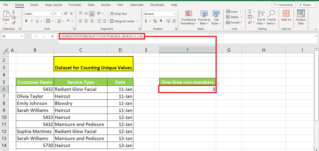
=SUM(IF(ISTEXT(B6:B14)*COUNTIF(B6:B14, B6:B14)=1,1,0))
Here’s the result:
These formulas will count how many unique values are present in your list, but they won’t tell you what these unique values are.
Using the UNIQUE function
The formulas in the first two methods only count how many unique values are present in your list but won’t tell you what these unique values are.
The unique function is a simple way to get a list of the unique values.
Step 1: Use the UNIQUE formula
Simply write this formula for your data:
=UNIQUE({Column array})
=UNIQUE(B6:B14)
Here’s how it works for our dataset:
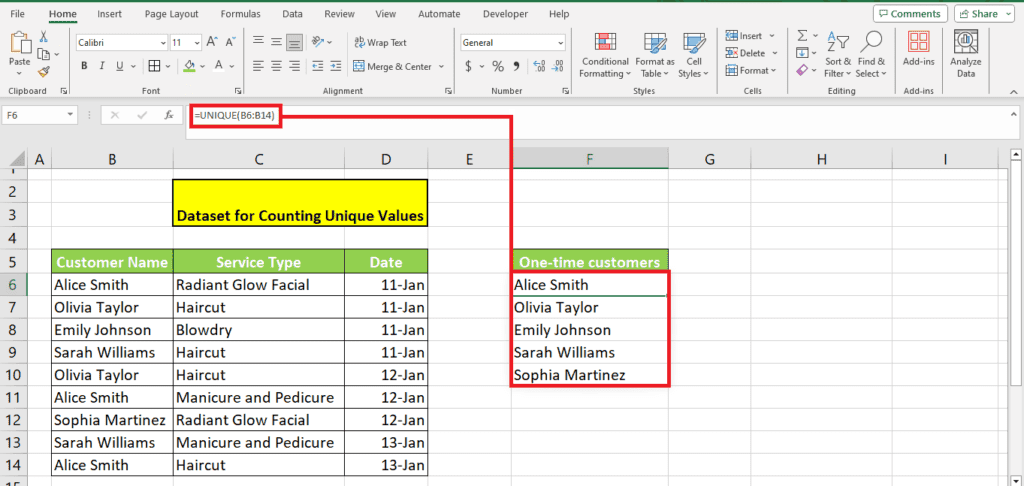
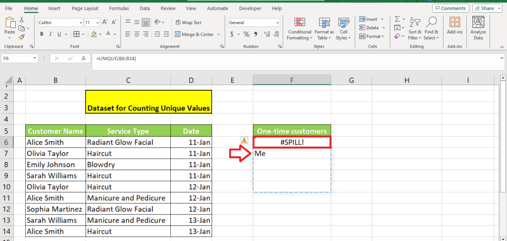
Note: This formula will create an array. If you attempt to change any cell in this array, it will show a #SPILL error:
Step 2: Adding TRUE to the UNIQUE function
The UNIQUE function returns all the distinct values in the list. This means we have a list of all the customers who availed services, regardless of how many times.
To get this formula to return only those unique values that occur once in the dataset, here’s the modified formula to use:
=UNIQUE({Column array},,TRUE)
=UNIQUE(B6:B14,,TRUE)
Here’s the result:
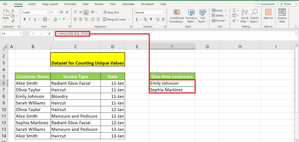
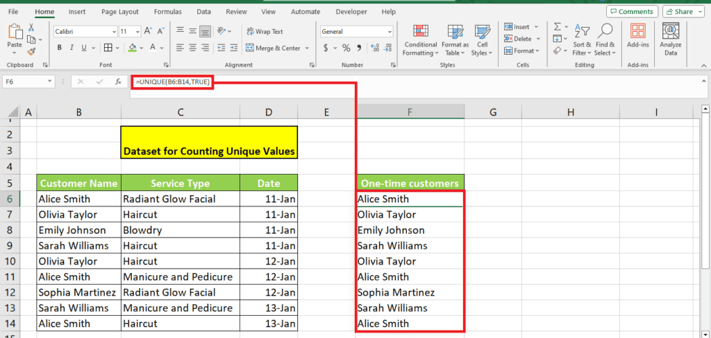
Note: This formula has two commas. If you enter just a single comma in the formula, it will return all the values in the column as it is:
Step 3: Count the unique values
The simple UNIQUE function returns a list of the distinct entries in the dataset. But if you only wish to get a number, there’s a way to count using this function.
Here’s the modified formula for this purpose:
=COUNTA(UNIQUE({Column array}))
=COUNTA(UNIQUE(B6:B14))
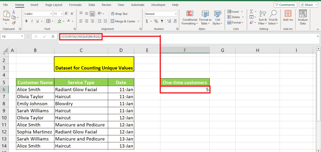
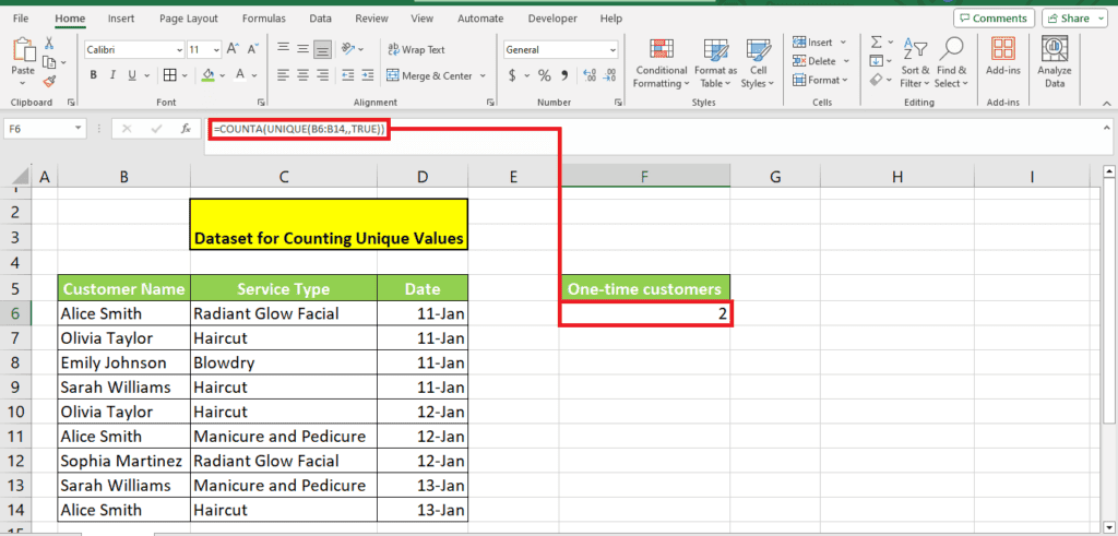
Additionally, by adding TRUE in the function, you can get the number of unique values in the list – the values that occur only once.
Here’s the formula:
=COUNTA(UNIQUE({Column array},,TRUE))
=COUNTA(UNIQUE(B6:B14,,TRUE))
Here’s the result:
Using the Advanced Filter option
The Advanced Filter option is the fourth way to get a list of distinct records from your table.
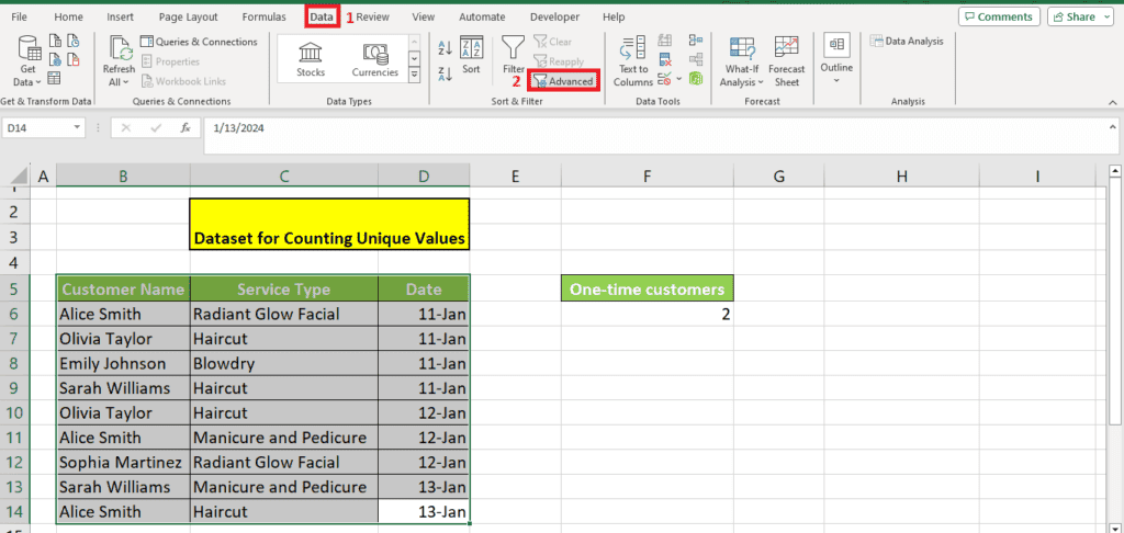
Step 1: Choose the Advanced Filter
The first step is to head to the Data tab from the top ribbon and locate ‘Advanced’ under the ‘Sort & Filter’ options.
Step 2: Enter the details
In the window that pops up, select your column. Then, choose another location to copy the filtered table.
Check the option ‘Unique records only.’
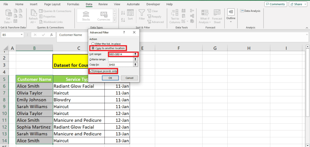
Here’s the result:
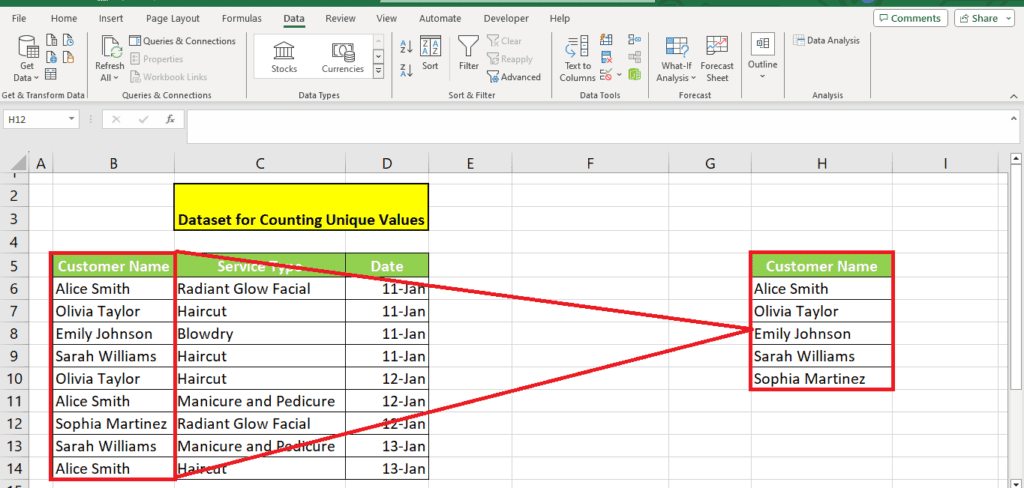
Using the filter for unique values
A simple trick to see the number of unique values in your table is to apply the filter.
Step 1: Apply a filter on your table
Click on any cell on your table. Then head to Data > Filter (under the ‘Sort & Filter’ options)
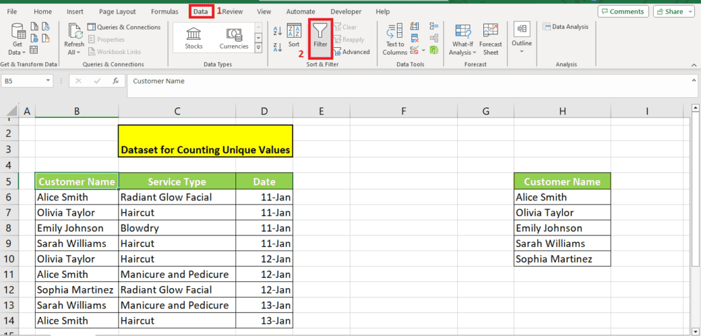
Step 2: Click the filter icon
Clicking this Filter option will add small arrows on the top label row. You can click the triangle icon on your desired column to see the unique records in your table.
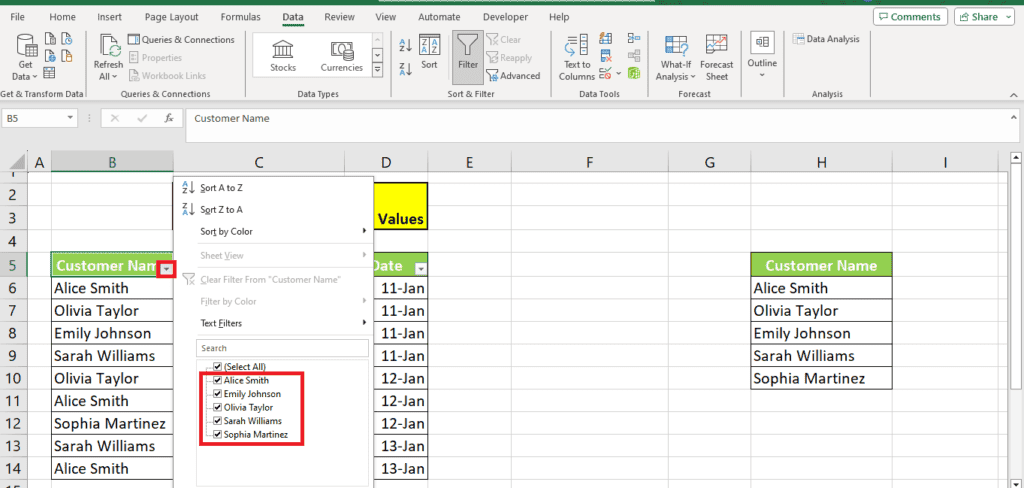
You can then select individual customer names and check how many times they are listed on the table.
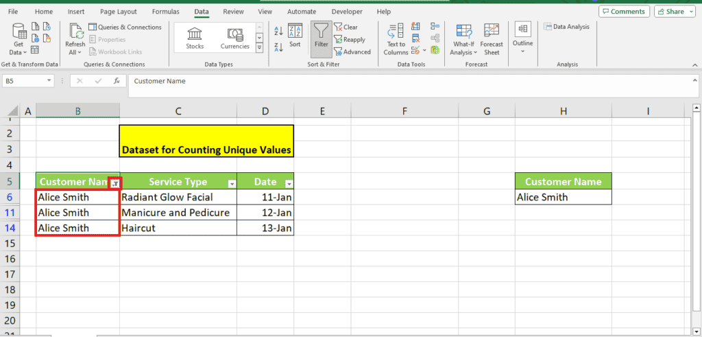
For instance, we want to see how often customer ‘Alice Smith’ has visited the salon.
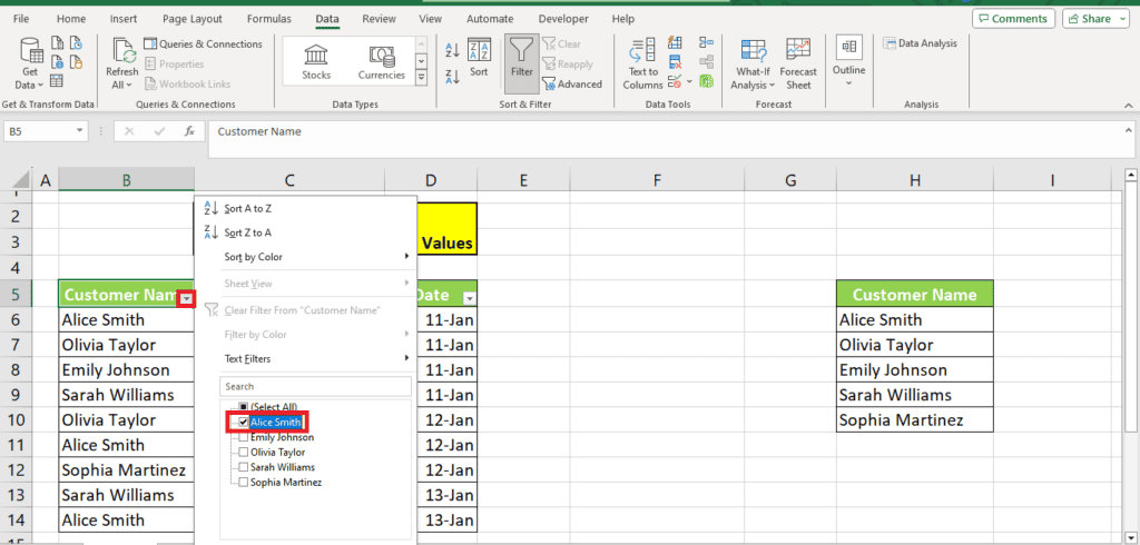
We only select ‘Alice Smith’ from the list, then click ‘OK.’
We see that customer ‘Alice’ visited three times in the month.
Frequently asked questions
What is the difference between unique and distinct values in Excel?
In Excel, unique values refer to values that occur just once in the data. On the other hand, distinct values are all the values listed in the table, regardless of the number of times they are repeated.
Wrapping up
The five methods mentioned in this guide are some ways to count the number of unique or distinct values within a given list. Combining these tricks with other functions will allow you to see exactly what the unique values in your data set are, as well as how many of them are present. This is also very helpful for companies and individuals looking for anomalous data or trying to understand recent trends across a data set.
If you’re want to expand your Excel knowledge, check out some of in-depth guides below.