TensorFlow प्रायिकता का भ्रमण (original) (raw)
इस Colab में, हम TensorFlow प्रायिकता की कुछ मूलभूत विशेषताओं का पता लगाते हैं।
निर्भरता और पूर्वापेक्षाएँ
आयात
from pprint import pprint
import matplotlib.pyplot as plt
import numpy as np
import seaborn as sns

import tensorflow.compat.v2 as tf
tf.enable_v2_behavior()

import tensorflow_probability as tfp

sns.reset_defaults()
sns.set_context(context='talk',font_scale=0.7)
plt.rcParams['image.cmap'] = 'viridis'

%matplotlib inline

tfd = tfp.distributions
tfb = tfp.bijectors
Utils
def print_subclasses_from_module(module, base_class, maxwidth=80):
  import functools, inspect, sys
  subclasses = [name for name, obj in inspect.getmembers(module)
                if inspect.isclass(obj) and issubclass(obj, base_class)]
  def red(acc, x):
    if not acc or len(acc[-1]) + len(x) + 2 > maxwidth:
      acc.append(x)
    else:
      acc[-1] += ", " + x
    return acc
  print('\n'.join(functools.reduce(red, subclasses, [])))
रेखांकित करें
- टेंसरफ्लो
- TensorFlow संभावना
- वितरण
- बिजेक्टर
- एमसीएमसी
- ...और अधिक!
प्रस्तावना: टेंसरफ्लो
TensorFlow एक वैज्ञानिक कंप्यूटिंग लाइब्रेरी है।
यह समर्थन करता है
- बहुत सारे गणितीय संचालन
- कुशल वेक्टरकृत गणना
- आसान हार्डवेयर त्वरण
- स्वचालित भेदभाव
वेक्टरीकरण
- वेक्टराइजेशन चीजों को तेज बनाता है!
- इसका मतलब यह भी है कि हम आकृतियों के बारे में बहुत सोचते हैं
mats = tf.random.uniform(shape=[1000, 10, 10])
vecs = tf.random.uniform(shape=[1000, 10, 1])

def for_loop_solve():
  return np.array(
    [tf.linalg.solve(mats[i, ...], vecs[i, ...]) for i in range(1000)])

def vectorized_solve():
  return tf.linalg.solve(mats, vecs)

# Vectorization for the win!
%timeit for_loop_solve()
%timeit vectorized_solve()
1 loops, best of 3: 2 s per loop 1000 loops, best of 3: 653 µs per loop
हार्डवेयर का त्वरण
# Code can run seamlessly on a GPU, just change Colab runtime type
# in the 'Runtime' menu.
if tf.test.gpu_device_name() == '/device:GPU:0':
  print("Using a GPU")
else:
  print("Using a CPU")
Using a CPU
स्वचालित भेदभाव
a = tf.constant(np.pi)
b = tf.constant(np.e)
with tf.GradientTape() as tape:
  tape.watch([a, b])
  c = .5 * (a**2 + b**2)
grads = tape.gradient(c, [a, b])
print(grads[0])
print(grads[1])
tf.Tensor(3.1415927, shape=(), dtype=float32) tf.Tensor(2.7182817, shape=(), dtype=float32)
TensorFlow संभावना
TensorFlow Probability TensorFlow में संभाव्य तर्क और सांख्यिकीय विश्लेषण के लिए एक पुस्तकालय है।
हम निम्न स्तर मॉड्यूलर घटकों की संरचना के माध्यम से मॉडलिंग, अनुमान, और आलोचना समर्थन करते हैं।
निम्न-स्तरीय बिल्डिंग ब्लॉक्स
- वितरण
- बिजेक्टर
उच्च (एर) -लेवल निर्माण
- मार्कोव चेन मोंटे कार्लोस
- संभाव्य परतें
- संरचनात्मक समय श्रृंखला
- सामान्यीकृत रैखिक मॉडल
- अनुकूलक
वितरण
एक tfp.distributions.Distribution : दो प्रमुख तरीकों के साथ एक वर्ग है sample और log_prob ।
TFP के बहुत सारे वितरण हैं!
print_subclasses_from_module(tfp.distributions, tfp.distributions.Distribution)
Autoregressive, BatchReshape, Bates, Bernoulli, Beta, BetaBinomial, Binomial Blockwise, Categorical, Cauchy, Chi, Chi2, CholeskyLKJ, ContinuousBernoulli Deterministic, Dirichlet, DirichletMultinomial, Distribution, DoublesidedMaxwell Empirical, ExpGamma, ExpRelaxedOneHotCategorical, Exponential, FiniteDiscrete Gamma, GammaGamma, GaussianProcess, GaussianProcessRegressionModel GeneralizedNormal, GeneralizedPareto, Geometric, Gumbel, HalfCauchy, HalfNormal HalfStudentT, HiddenMarkovModel, Horseshoe, Independent, InverseGamma InverseGaussian, JohnsonSU, JointDistribution, JointDistributionCoroutine JointDistributionCoroutineAutoBatched, JointDistributionNamed JointDistributionNamedAutoBatched, JointDistributionSequential JointDistributionSequentialAutoBatched, Kumaraswamy, LKJ, Laplace LinearGaussianStateSpaceModel, LogLogistic, LogNormal, Logistic, LogitNormal Mixture, MixtureSameFamily, Moyal, Multinomial, MultivariateNormalDiag MultivariateNormalDiagPlusLowRank, MultivariateNormalFullCovariance MultivariateNormalLinearOperator, MultivariateNormalTriL MultivariateStudentTLinearOperator, NegativeBinomial, Normal, OneHotCategorical OrderedLogistic, PERT, Pareto, PixelCNN, PlackettLuce, Poisson PoissonLogNormalQuadratureCompound, PowerSpherical, ProbitBernoulli QuantizedDistribution, RelaxedBernoulli, RelaxedOneHotCategorical, Sample SinhArcsinh, SphericalUniform, StudentT, StudentTProcess TransformedDistribution, Triangular, TruncatedCauchy, TruncatedNormal, Uniform VariationalGaussianProcess, VectorDeterministic, VonMises VonMisesFisher, Weibull, WishartLinearOperator, WishartTriL, Zipf
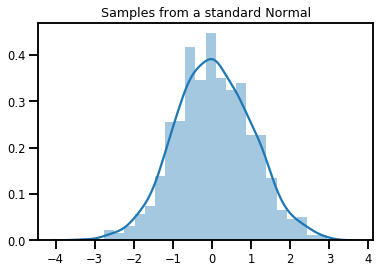
एक साधारण अदिश-variate Distribution
# A standard normal
normal = tfd.Normal(loc=0., scale=1.)
print(normal)
tfp.distributions.Normal("Normal", batch_shape=[], event_shape=[], dtype=float32)
# Plot 1000 samples from a standard normal
samples = normal.sample(1000)
sns.distplot(samples)
plt.title("Samples from a standard Normal")
plt.show()
# Compute the log_prob of a point in the event space of `normal`
normal.log_prob(0.)
<tf.Tensor: shape=(), dtype=float32, numpy=-0.9189385>
# Compute the log_prob of a few points
normal.log_prob([-1., 0., 1.])
<tf.Tensor: shape=(3,), dtype=float32, numpy=array([-1.4189385, -0.9189385, -1.4189385], dtype=float32)>
वितरण और आकार
Numpy ndarrays और TensorFlow Tensors आकार की है।
TensorFlow संभावना Distributions भले ही स्मृति का एक ही हिस्सा (शब्दार्थ अलग टुकड़ों में हम विभाजन आकार, - आकार अर्थ विज्ञान है Tensor / ndarray ) पूरे सब कुछ के लिए प्रयोग किया जाता है।
- बैच आकार का एक संग्रह को दर्शाता
Distributionअलग मानकों के साथ रों - घटना आकार से नमूने के आकार को दर्शाता
Distribution।
हम हमेशा "बाएं" पर बैच आकार और "दाएं" पर ईवेंट आकार डालते हैं।
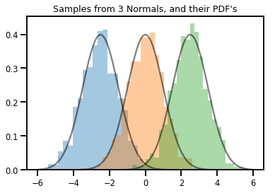
अदिश-variate का एक बैच Distributions
बैच "सदिश" वितरण की तरह हैं: स्वतंत्र उदाहरण जिनकी गणना समानांतर में होती है।
# Create a batch of 3 normals, and plot 1000 samples from each
normals = tfd.Normal([-2.5, 0., 2.5], 1.)  # The scale parameter broadacasts!
print("Batch shape:", normals.batch_shape)
print("Event shape:", normals.event_shape)
Batch shape: (3,) Event shape: ()
# Samples' shapes go on the left!
samples = normals.sample(1000)
print("Shape of samples:", samples.shape)
Shape of samples: (1000, 3)
# Sample shapes can themselves be more complicated
print("Shape of samples:", normals.sample([10, 10, 10]).shape)
Shape of samples: (10, 10, 10, 3)
# A batch of normals gives a batch of log_probs.
print(normals.log_prob([-2.5, 0., 2.5]))
tf.Tensor([-0.9189385 -0.9189385 -0.9189385], shape=(3,), dtype=float32)
# The computation broadcasts, so a batch of normals applied to a scalar
# also gives a batch of log_probs.
print(normals.log_prob(0.))
tf.Tensor([-4.0439386 -0.9189385 -4.0439386], shape=(3,), dtype=float32)
# Normal numpy-like broadcasting rules apply!
xs = np.linspace(-6, 6, 200)
try:
  normals.log_prob(xs)
except Exception as e:
  print("TFP error:", e.message)
TFP error: Incompatible shapes: [200] vs. [3] [Op:SquaredDifference]
# That fails for the same reason this does:
try:
  np.zeros(200) + np.zeros(3)
except Exception as e:
  print("Numpy error:", e)
Numpy error: operands could not be broadcast together with shapes (200,) (3,)
# But this would work:
a = np.zeros([200, 1]) + np.zeros(3)
print("Broadcast shape:", a.shape)
Broadcast shape: (200, 3)
# And so will this!
xs = np.linspace(-6, 6, 200)[..., np.newaxis]
# => shape = [200, 1]

lps = normals.log_prob(xs)
print("Broadcast log_prob shape:", lps.shape)
Broadcast log_prob shape: (200, 3)
# Summarizing visually
for i in range(3):
  sns.distplot(samples[:, i], kde=False, norm_hist=True)
plt.plot(np.tile(xs, 3), normals.prob(xs), c='k', alpha=.5)
plt.title("Samples from 3 Normals, and their PDF's")
plt.show()
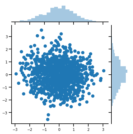
एक वेक्टर variate Distribution
mvn = tfd.MultivariateNormalDiag(loc=[0., 0.], scale_diag = [1., 1.])
print("Batch shape:", mvn.batch_shape)
print("Event shape:", mvn.event_shape)
Batch shape: () Event shape: (2,)
samples = mvn.sample(1000)
print("Samples shape:", samples.shape)
Samples shape: (1000, 2)
g = sns.jointplot(samples[:, 0], samples[:, 1], kind='scatter')
plt.show()
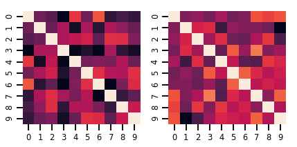
एक मैट्रिक्स-variate Distribution
lkj = tfd.LKJ(dimension=10, concentration=[1.5, 3.0])
print("Batch shape: ", lkj.batch_shape)
print("Event shape: ", lkj.event_shape)
Batch shape: (2,) Event shape: (10, 10)
samples = lkj.sample()
print("Samples shape: ", samples.shape)
Samples shape: (2, 10, 10)
fig, axes = plt.subplots(nrows=1, ncols=2, figsize=(6, 3))
sns.heatmap(samples[0, ...], ax=axes[0], cbar=False)
sns.heatmap(samples[1, ...], ax=axes[1], cbar=False)
fig.tight_layout()
plt.show()
गाऊसी प्रक्रियाएं
kernel = tfp.math.psd_kernels.ExponentiatedQuadratic()
xs = np.linspace(-5., 5., 200).reshape([-1, 1])
gp = tfd.GaussianProcess(kernel, index_points=xs)
print("Batch shape:", gp.batch_shape)
print("Event shape:", gp.event_shape)
Batch shape: () Event shape: (200,)
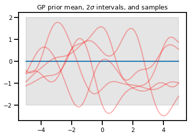
upper, lower = gp.mean() + [2 * gp.stddev(), -2 * gp.stddev()]
plt.plot(xs, gp.mean())
plt.fill_between(xs[..., 0], upper, lower, color='k', alpha=.1)
for _ in range(5):
  plt.plot(xs, gp.sample(), c='r', alpha=.3)
plt.title(r"GP prior mean, <span class="katex"><span class="katex-mathml"><math xmlns="http://www.w3.org/1998/Math/MathML"><semantics><mrow><mn>2</mn><mi>σ</mi></mrow><annotation encoding="application/x-tex">2\sigma</annotation></semantics></math></span><span class="katex-html" aria-hidden="true"><span class="base"><span class="strut" style="height:0.6444em;"></span><span class="mord">2</span><span class="mord mathnormal" style="margin-right:0.03588em;">σ</span></span></span></span> intervals, and samples")
plt.show()

#    *** Bonus question ***
# Why do so many of these functions lie outside the 95% intervals?
जीपी प्रतिगमन
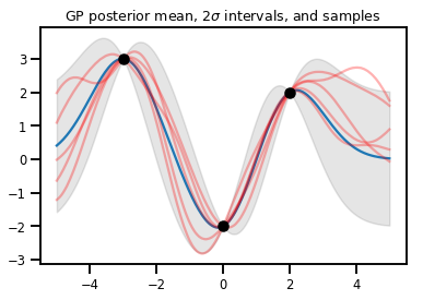
# Suppose we have some observed data
obs_x = [[-3.], [0.], [2.]]  # Shape 3x1 (3 1-D vectors)
obs_y = [3., -2., 2.]        # Shape 3   (3 scalars)

gprm = tfd.GaussianProcessRegressionModel(kernel, xs, obs_x, obs_y)
upper, lower = gprm.mean() + [2 * gprm.stddev(), -2 * gprm.stddev()]
plt.plot(xs, gprm.mean())
plt.fill_between(xs[..., 0], upper, lower, color='k', alpha=.1)
for _ in range(5):
  plt.plot(xs, gprm.sample(), c='r', alpha=.3)
plt.scatter(obs_x, obs_y, c='k', zorder=3)
plt.title(r"GP posterior mean, <span class="katex"><span class="katex-mathml"><math xmlns="http://www.w3.org/1998/Math/MathML"><semantics><mrow><mn>2</mn><mi>σ</mi></mrow><annotation encoding="application/x-tex">2\sigma</annotation></semantics></math></span><span class="katex-html" aria-hidden="true"><span class="base"><span class="strut" style="height:0.6444em;"></span><span class="mord">2</span><span class="mord mathnormal" style="margin-right:0.03588em;">σ</span></span></span></span> intervals, and samples")
plt.show()
बिजेक्टर
बिजेक्टर (ज्यादातर) उलटा, सुचारू कार्यों का प्रतिनिधित्व करते हैं। उनका उपयोग वितरण को बदलने, नमूने लेने और log_probs की गणना करने की क्षमता को संरक्षित करने के लिए किया जा सकता है। वे में हो सकता है tfp.bijectors मॉड्यूल।
प्रत्येक बायजेक्टर कम से कम 3 विधियों को लागू करता है:
forward,inverse, और- (कम से कम) में से एक
forward_log_det_jacobianऔरinverse_log_det_jacobian।
इन अवयवों के साथ, हम एक वितरण को बदल सकते हैं और फिर भी परिणाम से नमूने और लॉग जांच प्राप्त कर सकते हैं!
गणित में, कुछ सुस्ती से
- \(X\) पीडीएफ के साथ एक यादृच्छिक चर है \(p(x)\)
- \(g\) के स्थान पर एक चिकनी, उलटी समारोह है \(X\)की
- \(Y = g(X)\) एक नया, तब्दील यादृच्छिक चर है
- \(p(Y=y) = p(X=g^{-1}(y)) \cdot |\nabla g^{-1}(y)|\)
कैशिंग
बायजेक्टर फॉरवर्ड और इनवर्स कंप्यूटेशंस को भी कैश करते हैं, और लॉग-डेट-जैकोबियन, जो हमें संभावित रूप से बहुत महंगे ऑपरेशन को दोहराने की अनुमति देता है!
print_subclasses_from_module(tfp.bijectors, tfp.bijectors.Bijector)
AbsoluteValue, Affine, AffineLinearOperator, AffineScalar, BatchNormalization Bijector, Blockwise, Chain, CholeskyOuterProduct, CholeskyToInvCholesky CorrelationCholesky, Cumsum, DiscreteCosineTransform, Exp, Expm1, FFJORD FillScaleTriL, FillTriangular, FrechetCDF, GeneralizedExtremeValueCDF GeneralizedPareto, GompertzCDF, GumbelCDF, Identity, Inline, Invert IteratedSigmoidCentered, KumaraswamyCDF, LambertWTail, Log, Log1p MaskedAutoregressiveFlow, MatrixInverseTriL, MatvecLU, MoyalCDF, NormalCDF Ordered, Pad, Permute, PowerTransform, RationalQuadraticSpline, RayleighCDF RealNVP, Reciprocal, Reshape, Scale, ScaleMatvecDiag, ScaleMatvecLU ScaleMatvecLinearOperator, ScaleMatvecTriL, ScaleTriL, Shift, ShiftedGompertzCDF Sigmoid, Sinh, SinhArcsinh, SoftClip, Softfloor, SoftmaxCentered, Softplus Softsign, Split, Square, Tanh, TransformDiagonal, Transpose, WeibullCDF
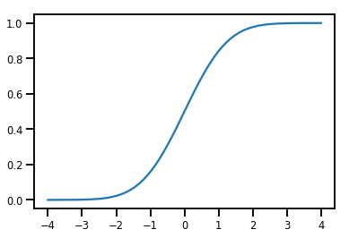
एक साधारण Bijector
normal_cdf = tfp.bijectors.NormalCDF()
xs = np.linspace(-4., 4., 200)
plt.plot(xs, normal_cdf.forward(xs))
plt.show()
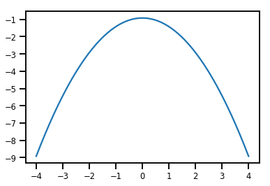
plt.plot(xs, normal_cdf.forward_log_det_jacobian(xs, event_ndims=0))
plt.show()
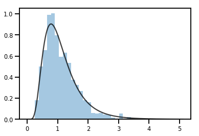
एक Bijector एक बदलने Distribution
exp_bijector = tfp.bijectors.Exp()
log_normal = exp_bijector(tfd.Normal(0., .5))

samples = log_normal.sample(1000)
xs = np.linspace(1e-10, np.max(samples), 200)
sns.distplot(samples, norm_hist=True, kde=False)
plt.plot(xs, log_normal.prob(xs), c='k', alpha=.75)
plt.show()
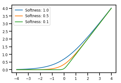
बैचिंग Bijectors
# Create a batch of bijectors of shape [3,]
softplus = tfp.bijectors.Softplus(
  hinge_softness=[1., .5, .1])
print("Hinge softness shape:", softplus.hinge_softness.shape)
Hinge softness shape: (3,)
# For broadcasting, we want this to be shape [200, 1]
xs = np.linspace(-4., 4., 200)[..., np.newaxis]
ys = softplus.forward(xs)
print("Forward shape:", ys.shape)
Forward shape: (200, 3)
# Visualization
lines = plt.plot(np.tile(xs, 3), ys)
for line, hs in zip(lines, softplus.hinge_softness):
  line.set_label("Softness: %1.1f" % hs)
plt.legend()
plt.show()
कैशिंग
# This bijector represents a matrix outer product on the forward pass,
# and a cholesky decomposition on the inverse pass. The latter costs O(N^3)!
bij = tfb.CholeskyOuterProduct()

size = 2500
# Make a big, lower-triangular matrix
big_lower_triangular = tf.eye(size)
# Squaring it gives us a positive-definite matrix
big_positive_definite = bij.forward(big_lower_triangular)

# Caching for the win!
%timeit bij.inverse(big_positive_definite)
%timeit tf.linalg.cholesky(big_positive_definite)
10000 loops, best of 3: 114 µs per loop 1 loops, best of 3: 208 ms per loop
एमसीएमसी
TFP ने हैमिल्टनियन मोंटे कार्लो सहित कुछ मानक मार्कोव श्रृंखला मोंटे कार्लो एल्गोरिदम के समर्थन में बनाया है।
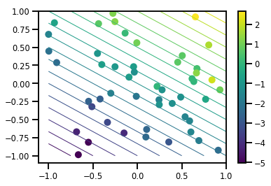
एक डेटा सेट उत्पन्न करें
# Generate some data
def f(x, w):
  # Pad x with 1's so we can add bias via matmul
  x = tf.pad(x, [[1, 0], [0, 0]], constant_values=1)
  linop = tf.linalg.LinearOperatorFullMatrix(w[..., np.newaxis])
  result = linop.matmul(x, adjoint=True)
  return result[..., 0, :]

num_features = 2
num_examples = 50
noise_scale = .5
true_w = np.array([-1., 2., 3.])

xs = np.random.uniform(-1., 1., [num_features, num_examples])
ys = f(xs, true_w) + np.random.normal(0., noise_scale, size=num_examples)
# Visualize the data set
plt.scatter(*xs, c=ys, s=100, linewidths=0)

grid = np.meshgrid(*([np.linspace(-1, 1, 100)] * 2))
xs_grid = np.stack(grid, axis=0)
fs_grid = f(xs_grid.reshape([num_features, -1]), true_w)
fs_grid = np.reshape(fs_grid, [100, 100])
plt.colorbar()
plt.contour(xs_grid[0, ...], xs_grid[1, ...], fs_grid, 20, linewidths=1)
plt.show()
हमारे संयुक्त लॉग-प्रोब फ़ंक्शन को परिभाषित करें
Unnormalized पीछे डेटा पर बंद करने के लिए एक के रूप में करने का परिणाम है आंशिक आवेदन संयुक्त लॉग समस्या की।
# Define the joint_log_prob function, and our unnormalized posterior.
def joint_log_prob(w, x, y):
  # Our model in maths is
  #   w ~ MVN([0, 0, 0], diag([1, 1, 1]))
  #   y_i ~ Normal(w @ x_i, noise_scale),  i=1..N

  rv_w = tfd.MultivariateNormalDiag(
    loc=np.zeros(num_features + 1),
    scale_diag=np.ones(num_features + 1))

  rv_y = tfd.Normal(f(x, w), noise_scale)
  return (rv_w.log_prob(w) +
          tf.reduce_sum(rv_y.log_prob(y), axis=-1))
# Create our unnormalized target density by currying x and y from the joint.
def unnormalized_posterior(w):
  return joint_log_prob(w, xs, ys)
एचएमसी ट्रांजिशन कर्नेल बनाएं और नमूना_चैन पर कॉल करें
# Create an HMC TransitionKernel
hmc_kernel = tfp.mcmc.HamiltonianMonteCarlo(
  target_log_prob_fn=unnormalized_posterior,
  step_size=np.float64(.1),
  num_leapfrog_steps=2)
# We wrap sample_chain in tf.function, telling TF to precompile a reusable
# computation graph, which will dramatically improve performance.
@tf.function
def run_chain(initial_state, num_results=1000, num_burnin_steps=500):
  return tfp.mcmc.sample_chain(
    num_results=num_results,
    num_burnin_steps=num_burnin_steps,
    current_state=initial_state,
    kernel=hmc_kernel,
    trace_fn=lambda current_state, kernel_results: kernel_results)
initial_state = np.zeros(num_features + 1)
samples, kernel_results = run_chain(initial_state)
print("Acceptance rate:", kernel_results.is_accepted.numpy().mean())
Acceptance rate: 0.915
यह बढ़िया नहीं है! हम .65 के करीब एक स्वीकृति दर चाहते हैं।
(देखें "विभिन्न महानगरों-हेस्टिंग्स एल्गोरिदम के लिए इष्टतम स्केलिंग" , रॉबर्ट्स एंड Rosenthal, 2001)
अनुकूली चरण आकार
हम एक में हमारे एचएमसी TransitionKernel लपेट कर सकते हैं SimpleStepSizeAdaptation "मेटा-गिरी" है, जो कुछ (बल्कि सरल अनुमानी) तर्क बर्निं दौरान एचएमसी कदम आकार अनुकूल करने के लिए लागू होगी। हम चरण आकार को अनुकूलित करने के लिए 80% बर्निन आवंटित करते हैं, और फिर शेष 20% को केवल मिश्रण करने के लिए जाने देते हैं।
# Apply a simple step size adaptation during burnin
@tf.function
def run_chain(initial_state, num_results=1000, num_burnin_steps=500):
  adaptive_kernel = tfp.mcmc.SimpleStepSizeAdaptation(
      hmc_kernel,
      num_adaptation_steps=int(.8 * num_burnin_steps),
      target_accept_prob=np.float64(.65))

  return tfp.mcmc.sample_chain(
    num_results=num_results,
    num_burnin_steps=num_burnin_steps,
    current_state=initial_state,
    kernel=adaptive_kernel,
    trace_fn=lambda cs, kr: kr)
samples, kernel_results = run_chain(
  initial_state=np.zeros(num_features+1))
print("Acceptance rate:", kernel_results.inner_results.is_accepted.numpy().mean())
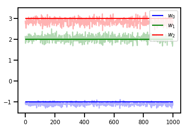
Acceptance rate: 0.634
# Trace plots
colors = ['b', 'g', 'r']
for i in range(3):
plt.plot(samples[:, i], c=colors[i], alpha=.3)
plt.hlines(true_w[i], 0, 1000, zorder=4, color=colors[i], label="$w_{}$".format(i))
plt.legend(loc='upper right')
plt.show()
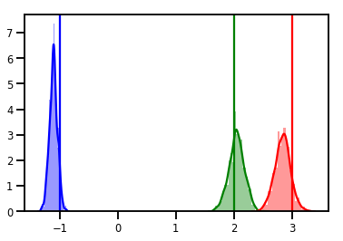
# Histogram of samples
for i in range(3):
sns.distplot(samples[:, i], color=colors[i])
ymax = plt.ylim()[1]
for i in range(3):
plt.vlines(true_w[i], 0, ymax, color=colors[i])
plt.ylim(0, ymax)
plt.show()
निदान
ट्रेस प्लॉट अच्छे हैं, लेकिन डायग्नोस्टिक्स अच्छे हैं!
पहले हमें कई चेन चलाने की जरूरत है। इस का एक बैच दे रही है के रूप में सरल रूप में है initial_state tensors।
# Instead of a single set of initial w's, we create a batch of 8.
num_chains = 8
initial_state = np.zeros([num_chains, num_features + 1])

chains, kernel_results = run_chain(initial_state)

r_hat = tfp.mcmc.potential_scale_reduction(chains)
print("Acceptance rate:", kernel_results.inner_results.is_accepted.numpy().mean())
print("R-hat diagnostic (per latent variable):", r_hat.numpy())
Acceptance rate: 0.59175 R-hat diagnostic (per latent variable): [0.99998395 0.99932185 0.9997064 ]
शोर पैमाने का नमूना लेना
# Define the joint_log_prob function, and our unnormalized posterior.
def joint_log_prob(w, sigma, x, y):
  # Our model in maths is
  #   w ~ MVN([0, 0, 0], diag([1, 1, 1]))
  #   y_i ~ Normal(w @ x_i, noise_scale),  i=1..N

  rv_w = tfd.MultivariateNormalDiag(
    loc=np.zeros(num_features + 1),
    scale_diag=np.ones(num_features + 1))

  rv_sigma = tfd.LogNormal(np.float64(1.), np.float64(5.))

  rv_y = tfd.Normal(f(x, w), sigma[..., np.newaxis])
  return (rv_w.log_prob(w) +
          rv_sigma.log_prob(sigma) +
          tf.reduce_sum(rv_y.log_prob(y), axis=-1))

# Create our unnormalized target density by currying x and y from the joint.
def unnormalized_posterior(w, sigma):
  return joint_log_prob(w, sigma, xs, ys)


# Create an HMC TransitionKernel
hmc_kernel = tfp.mcmc.HamiltonianMonteCarlo(
  target_log_prob_fn=unnormalized_posterior,
  step_size=np.float64(.1),
  num_leapfrog_steps=4)


# Create a TransformedTransitionKernl
transformed_kernel = tfp.mcmc.TransformedTransitionKernel(
    inner_kernel=hmc_kernel,
    bijector=[tfb.Identity(),    # w
              tfb.Invert(tfb.Softplus())])   # sigma


# Apply a simple step size adaptation during burnin
@tf.function
def run_chain(initial_state, num_results=1000, num_burnin_steps=500):
  adaptive_kernel = tfp.mcmc.SimpleStepSizeAdaptation(
      transformed_kernel,
      num_adaptation_steps=int(.8 * num_burnin_steps),
      target_accept_prob=np.float64(.75))

  return tfp.mcmc.sample_chain(
    num_results=num_results,
    num_burnin_steps=num_burnin_steps,
    current_state=initial_state,
    kernel=adaptive_kernel,
    seed=(0, 1),
    trace_fn=lambda cs, kr: kr)


# Instead of a single set of initial w's, we create a batch of 8.
num_chains = 8
initial_state = [np.zeros([num_chains, num_features + 1]),
                 .54 * np.ones([num_chains], dtype=np.float64)]

chains, kernel_results = run_chain(initial_state)

r_hat = tfp.mcmc.potential_scale_reduction(chains)
print("Acceptance rate:", kernel_results.inner_results.inner_results.is_accepted.numpy().mean())
print("R-hat diagnostic (per w variable):", r_hat[0].numpy())
print("R-hat diagnostic (sigma):", r_hat[1].numpy())
Acceptance rate: 0.715875 R-hat diagnostic (per w variable): [1.0000073 1.00458208 1.00450512] R-hat diagnostic (sigma): 1.0092056996149859
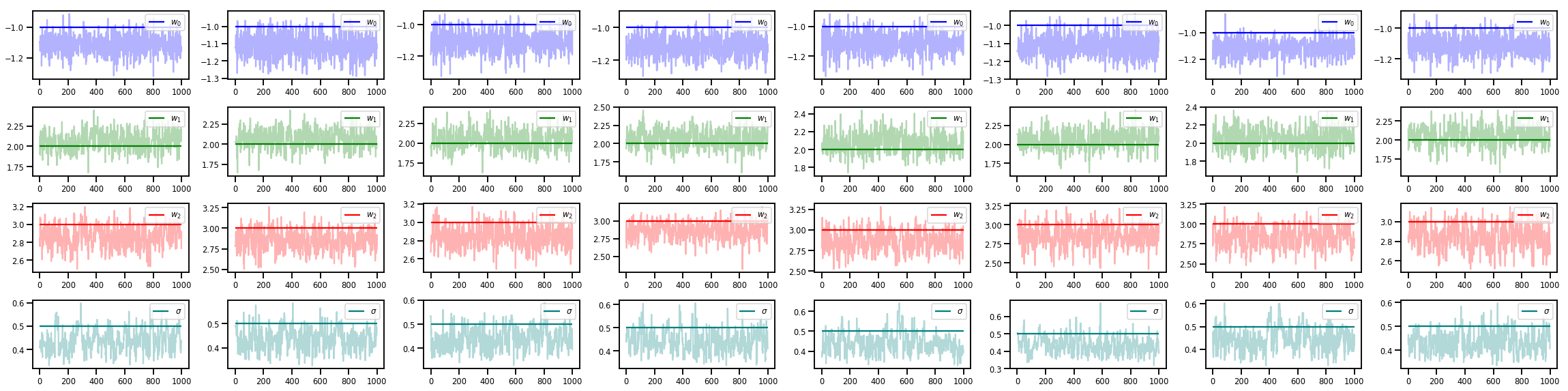
w_chains, sigma_chains = chains
# Trace plots of w (one of 8 chains)
colors = ['b', 'g', 'r', 'teal']
fig, axes = plt.subplots(4, num_chains, figsize=(4 * num_chains, 8))
for j in range(num_chains):
for i in range(3):
ax = axes[i][j]
ax.plot(w_chains[:, j, i], c=colors[i], alpha=.3)
ax.hlines(true_w[i], 0, 1000, zorder=4, color=colors[i], label="$w_{}$".format(i))
ax.legend(loc='upper right')
ax = axes[3][j]
ax.plot(sigma_chains[:, j], alpha=.3, c=colors[3])
ax.hlines(noise_scale, 0, 1000, zorder=4, color=colors[3], label=r"$\sigma$".format(i))
ax.legend(loc='upper right')
fig.tight_layout()
plt.show()
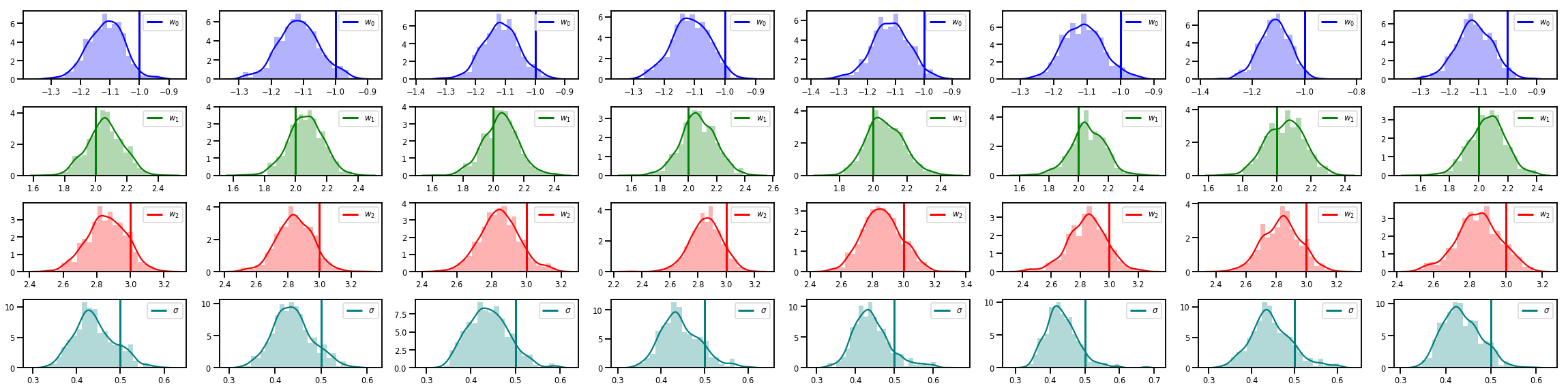
# Histogram of samples of w
fig, axes = plt.subplots(4, num_chains, figsize=(4 * num_chains, 8))
for j in range(num_chains):
for i in range(3):
ax = axes[i][j]
sns.distplot(w_chains[:, j, i], color=colors[i], norm_hist=True, ax=ax, hist_kws={'alpha': .3})
for i in range(3):
ax = axes[i][j]
ymax = ax.get_ylim()[1]
ax.vlines(true_w[i], 0, ymax, color=colors[i], label="$w_{}$".format(i), linewidth=3)
ax.set_ylim(0, ymax)
ax.legend(loc='upper right')
ax = axes[3][j]
sns.distplot(sigma_chains[:, j], color=colors[3], norm_hist=True, ax=ax, hist_kws={'alpha': .3})
ymax = ax.get_ylim()[1]
ax.vlines(noise_scale, 0, ymax, color=colors[3], label=r"$\sigma$".format(i), linewidth=3)
ax.set_ylim(0, ymax)
ax.legend(loc='upper right')
fig.tight_layout()
plt.show()
और भी बहुत कुछ है!
इन शानदार ब्लॉग पोस्ट और उदाहरणों को देखें:
- स्ट्रक्चरल समय श्रृंखला समर्थन ब्लॉग colab
- संभाव्य Keras परतें (इनपुट: टेन्सर, उत्पादन: वितरण!) ब्लॉग colab
- गाऊसी प्रक्रिया प्रतिगमन colab और अव्यक्त चर मॉडलिंग colab
अधिक उदाहरण और हमारे GitHub पर पुस्तिकाओं यहाँ !