Get Started with SCIntRuler (original) (raw)
Introducrtion
The accumulation of single-cell RNA-seq (scRNA-seq) studies highlights the potential benefits of integrating multiple data sets. By augmenting sample sizes and enhancing analytical robustness, integration can lead to more insightful biological conclusions. However, challenges arise due to the inherent diversity and batch discrepancies within and across studies. SCIntRuler, a novel R package, addresses these challenges by guiding the integration of multiple scRNA-seq data sets. SCIntRuler is an R package developed for single-cell RNA-seq analysis. It was designed using the Seurat framework, and offers existing and novel single-cell analytic work flows.
Integrating scRNA-seq data sets can be complex due to various factors, including batch effects and sample diversity. Key decisions – whether to integrate data sets, which method to choose for integration, and how to best handle inherent data discrepancies – are crucial.SCIntRuler offers a statistical metric to aid in these decisions, ensuring more robust and accurate analyses.
- Informed Decision Making: Helps researchers decide on the necessity of data integration and the most suitable method.
- Flexibility: Suitable for various scenarios, accommodating different levels of data heterogeneity.
- Robustness: Enhances analytical robustness in joint analyses of merged or integrated scRNA-seq data sets.
- User-Friendly: Streamlines decision-making processes, simplifying the complexities involved in scRNA-seq data integration.
1. Installation
To install the package, you need to install thebatchelor and MatrixGenerics package from Bioconductor.
# Check if BioManager is installed, install if not
if (!requireNamespace("BiocManager", quietly = TRUE))
    install.packages("BiocManager")

# Check if 'batchelor' is installed, install if not
if (!requireNamespace("batchelor", quietly = TRUE))
    BiocManager::install("batchelor")

# Check if 'MatrixGenerics' is installed, install if not
if (!requireNamespace("MatrixGenerics", quietly = TRUE))
    BiocManager::install("MatrixGenerics")
The SCIntRuler can be installed by the following commands, the source code can be found at GitHub.
After the installation, the package can be loaded with
2. Explore with an example data
Let’s start with an example data. We conducted a series of simulation studies to assess the efficacy of SCIntRuler in guiding the integration selection under different scenarios with varying degrees of shared information among data sets. We generated the simulation data based on a real Peripheral Blood Mononuclear Cells (PBMC)scRNA-seq dataset.
Overview of the data
This dataset is a subset of what we used in our Simulation 2, where we have three studies. In each study, we randomly drew different numbers of CD4 T helper cells, B cells, CD14 monocytes, and CD56 NK cells to mimic four real-world scenarios with three data sourcesSimulation 2 introduces a moderate overlap, with 20.3% cells sharing the same cell type identity. There are 2000 B cells and 400 CD4T cells in the first study, 700 CD14Mono cells and 400 CD4T cells in the second study, 2000 CD56NK cells and 400 CD4T cells in the third study. This data is already in Seurat format and can be found under /data. There are 32738 genes and 5900 cells in simulation 2. Here, we subset 800 cells with 3000 genes.
data("sim_data_sce", package = "SCIntRuler")
sim_data <- as.Seurat(sim_data_sce)
head(sim_data[[]])
#> orig.ident nCount_RNA nFeature_RNA CellType Study
#> AATTACGAATCGGT-1 SeuratProject 1035 365 Bcell Study1
#> AGAGCGGAGTCCTC-1 SeuratProject 1157 448 Bcell Study1
#> TTCTTACTGGTACT-1 SeuratProject 2824 884 Bcell Study1
#> TGACGCCTACACCA-1 SeuratProject 1801 644 Bcell Study1
#> ATTTGCACCTATGG-1 SeuratProject 2501 749 Bcell Study1
#> AGAACAGATGGAGG-1 SeuratProject 1113 391 Bcell Study1
#> RNA_snn_res.0.5 seurat_clusters ident
#> AATTACGAATCGGT-1 0 0 0
#> AGAGCGGAGTCCTC-1 0 0 0
#> TTCTTACTGGTACT-1 0 0 0
#> TGACGCCTACACCA-1 0 0 0
#> ATTTGCACCTATGG-1 0 0 0
#> AGAACAGATGGAGG-1 0 0 0Data pre-process and visulization with Seurat
Followed by the tutorial of Seurat, we first pre-processed the data by the functionsNormalizeData, FindVariableFeature,ScaleData, RunPCA, FindNeighbors,FinsClusters and RunUMAP fromSeurat and then draw the UMAP by using DimPlotstratified by Study and Cell Type.
# Normalize the data
sim_data <- NormalizeData(sim_data)
# Identify highly variable features
sim_data <- FindVariableFeatures(sim_data, selection.method = "vst", nfeatures = 2000)
# Scale the data
all.genes <- rownames(sim_data)
sim_data <- ScaleData(sim_data, features = all.genes)
# Perform linear dimensional reduction
sim_data <- RunPCA(sim_data, features = VariableFeatures(object = sim_data))
# Cluster the cells
sim_data <- FindNeighbors(sim_data, dims = 1:20)
sim_data <- FindClusters(sim_data, resolution = 0.5)
#> Modularity Optimizer version 1.3.0 by Ludo Waltman and Nees Jan van Eck
#>
#> Number of nodes: 800
#> Number of edges: 46490
#>
#> Running Louvain algorithm...
#> Maximum modularity in 10 random starts: 0.7653
#> Number of communities: 4
#> Elapsed time: 0 seconds
sim_data <- RunUMAP(sim_data, dims = 1:20)
UMAP separated by Study
p1 <- DimPlot(sim_data, reduction = "umap", label = FALSE, pt.size = .5, group.by = "Study", repel = TRUE)
p1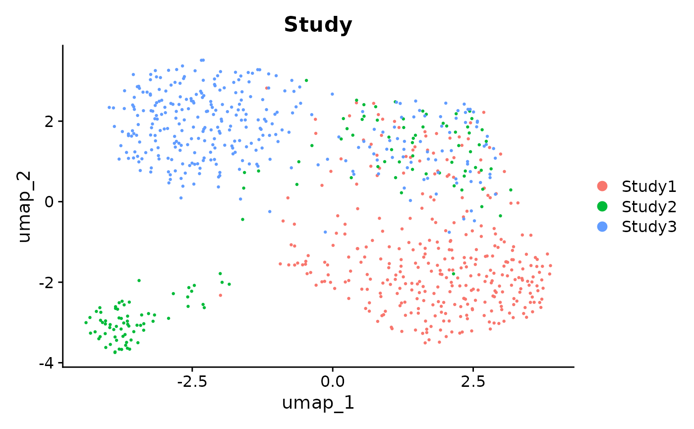
UMAP separated by cell type
p2 <- DimPlot(sim_data, reduction = "umap", label = TRUE, pt.size = .8, group.by = "CellType", repel = TRUE)
p2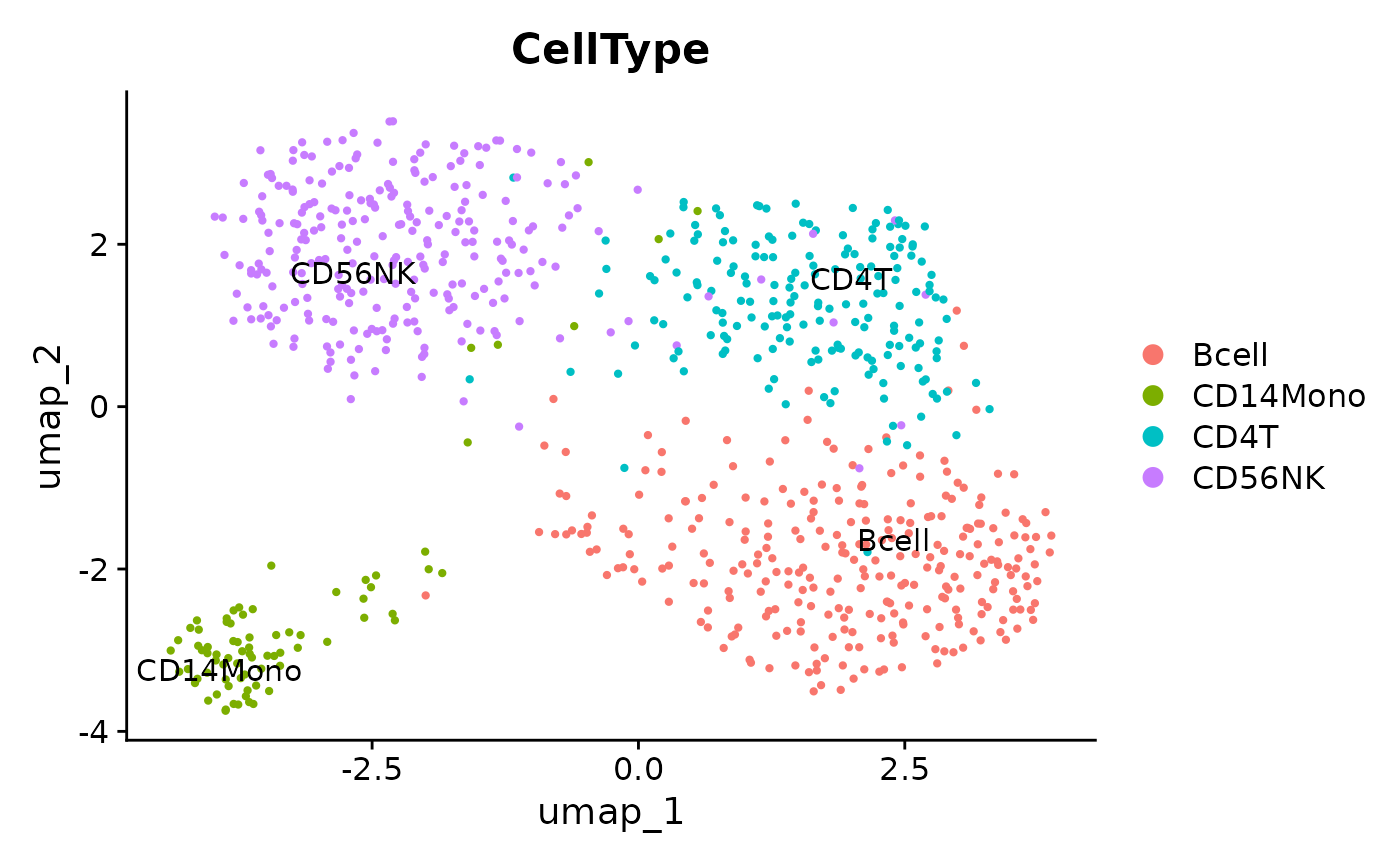
Try different data integration methods
To further illustrate which integration method is more suitable under different settings, we visualize the data without integration (simply merging the single cell objects) and after applying three popular data integration methods: CCA, Harmony and Scanorama. The UMAP visualizations across the simulations indicate that the choice of integration method significantly impacts the resulting data integration.
Run Seurat CCA
Seurat CCA can be directly applied by functionsFindIntegrationAnchors and IntegrateData inSeurat package. For more information, please seeTutorial of SeuratCCA.
### CCA
sim.list <- SplitObject(sim_data, split.by = "Study")
sim.anchors <- FindIntegrationAnchors(object.list = sim.list, dims = 1:30, reduction = "cca")

sim.int <- IntegrateData(anchorset = sim.anchors, dims = 1:30, new.assay.name = "CCA")
# run standard analysis workflow
sim.int <- ScaleData(sim.int, verbose = FALSE)
sim.int <- RunPCA(sim.int, npcs = 30, verbose = FALSE)
sim.int <- RunUMAP(sim.int, dims = 1:30, reduction.name = "umap_cca")
Run Harmony
Harmony is an algorithm for performing integration of single cell genomics data sets. To run harmony, we need to installharmony package. For more information, please see Quick start to Harmony.
### Harmony
# install.packages("harmony")

sim.harmony <- harmony::RunHarmony(sim_data, group.by.vars = "Study", reduction.use = "pca",
                                   #dims.use = 1:20, assay.use = "RNA"
    )

sim.int[["harmony"]] <- sim.harmony[["harmony"]]
sim.int <- RunUMAP(sim.int, dims = 1:20, reduction = "harmony", reduction.name = "umap_harmony")
UMAP figures for all integrated data
p5 <- DimPlot(sim_data, reduction = "umap", group.by = "Study") +
  theme(legend.position = "none",
        # axis.line.y = element_line( size = 2, linetype = "solid"),
        # axis.line.x = element_line( size = 2, linetype = "solid"),
        axis.text.y = element_text( color="black", size=20),
        axis.title.y = element_text(color="black", size=20),
        axis.text.x = element_text( color="black", size=20),
        axis.title.x = element_text(color="black", size=20))
p6 <- DimPlot(sim.int, reduction = "umap_cca", group.by = "Study") +
  theme(legend.position = "none",
        # axis.line.y = element_line( size = 2, linetype = "solid"),
        # axis.line.x = element_line( size = 2, linetype = "solid"),
        axis.text.y = element_text( color="black", size=20),
        axis.title.y = element_text(color="black", size=20),
        axis.text.x = element_text( color="black", size=20),
        axis.title.x = element_text(color="black", size=20))
p7 <- DimPlot(sim.int, reduction = "umap_harmony", group.by = "Study") +
  theme(legend.position = "none",
        # axis.line.y = element_line( size = 2, linetype = "solid"),
        # axis.line.x = element_line( size = 2, linetype = "solid"),
        axis.text.y = element_text( color="black", size=20),
        axis.title.y = element_text(color="black", size=20),
        axis.text.x = element_text( color="black", size=20),
        axis.title.x = element_text(color="black", size=20))

leg <- cowplot::get_legend(p5)
#> Warning in get_plot_component(plot, "guide-box"): Multiple components found;
#> returning the first one. To return all, use `return_all = TRUE`.
gridExtra::grid.arrange(gridExtra::arrangeGrob(p5 + NoLegend() + ggtitle("Unintegrated"),
                                               p6 + NoLegend() + ggtitle("Seurat CCA") ,
                                               p7 + NoLegend() + ggtitle("Harmony"),
                                               #p8 + NoLegend() + ggtitle("Scanorama"),
                                               nrow = 2),
    leg, ncol = 2, widths = c(20, 5))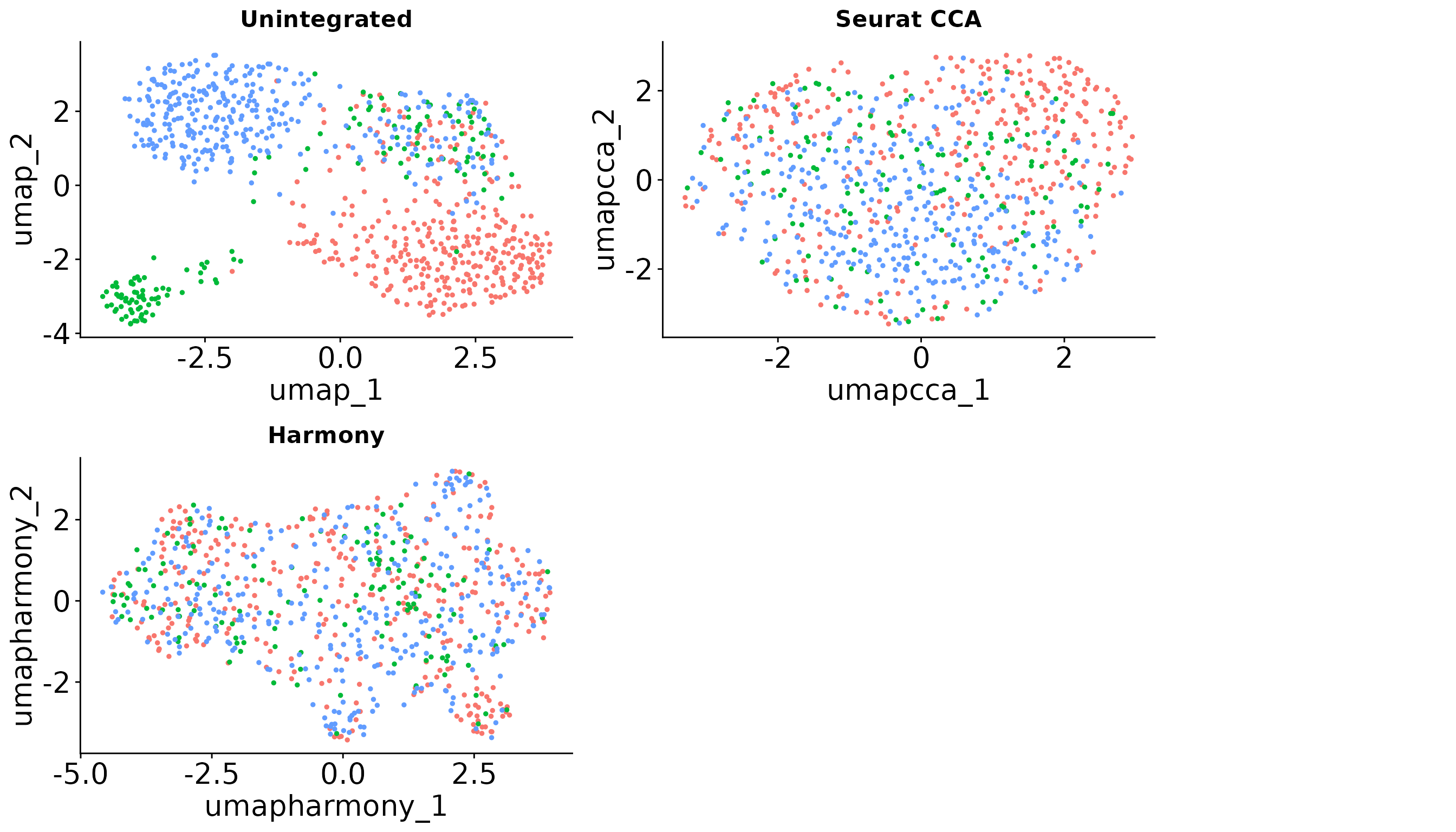
3. Applying SCIntRuler to example data
We first split the sim_data by Study and then run GetCluster and NormData to get Louvain clusters and normalized count matrix for each study. Furthermore, to perform the permutation test of relative-between cluster distance, FindNNDist can be then applied. We also have another function FindNNDistC that based onRcpp and C++ for faster matrix calculation.
sim.list <- SplitObject(sim_data, split.by = "Study")
fullcluster <- GetCluster(sim.list,50,200)
#> Modularity Optimizer version 1.3.0 by Ludo Waltman and Nees Jan van Eck
#>
#> Number of nodes: 336
#> Number of edges: 21610
#>
#> Running Louvain algorithm...
#> Maximum modularity in 10 random starts: 0.5099
#> Number of communities: 2
#> Elapsed time: 0 seconds
#> Modularity Optimizer version 1.3.0 by Ludo Waltman and Nees Jan van Eck
#>
#> Number of nodes: 136
#> Number of edges: 4813
#>
#> Running Louvain algorithm...
#> Maximum modularity in 10 random starts: 0.7201
#> Number of communities: 2
#> Elapsed time: 0 seconds
#> Modularity Optimizer version 1.3.0 by Ludo Waltman and Nees Jan van Eck
#>
#> Number of nodes: 328
#> Number of edges: 22343
#>
#> Running Louvain algorithm...
#> Maximum modularity in 10 random starts: 0.5141
#> Number of communities: 2
#> Elapsed time: 0 seconds

normCount <- NormData(sim.list)

#distmat <- FindNNDist(fullcluster, normCount, 20)
distmat <- FindNNDistC(fullcluster, normCount, 20)
#>   |                                                                    |                                                            |   0%  |                                                                    |====================                                        |  33%  |                                                                    |========================================                    |  67%  |                                                                    |============================================================| 100%
Calculate SCIntRuler and and an associated visualization
In this example data, we got a SCIntRuler score of 0.57, there is a noticeable but not large overlap of cell types across the data sets, showing a moderate level of shared information. The integration is essential to adjust for these effects and align the shared cell populations, ensuring that the integrated dataset accurately reflects the biological composition. Thus, the methods which can offer a balance between correcting for batch effects and maintaining biological variation would be the best. The UMAP visualizations across the simulations indicate that the choice of integration method significantly impacts the resulting data integration.
testres <- PermTest(fullcluster,distmat,15)
PlotSCIR(fullcluster,sim.list,testres,"")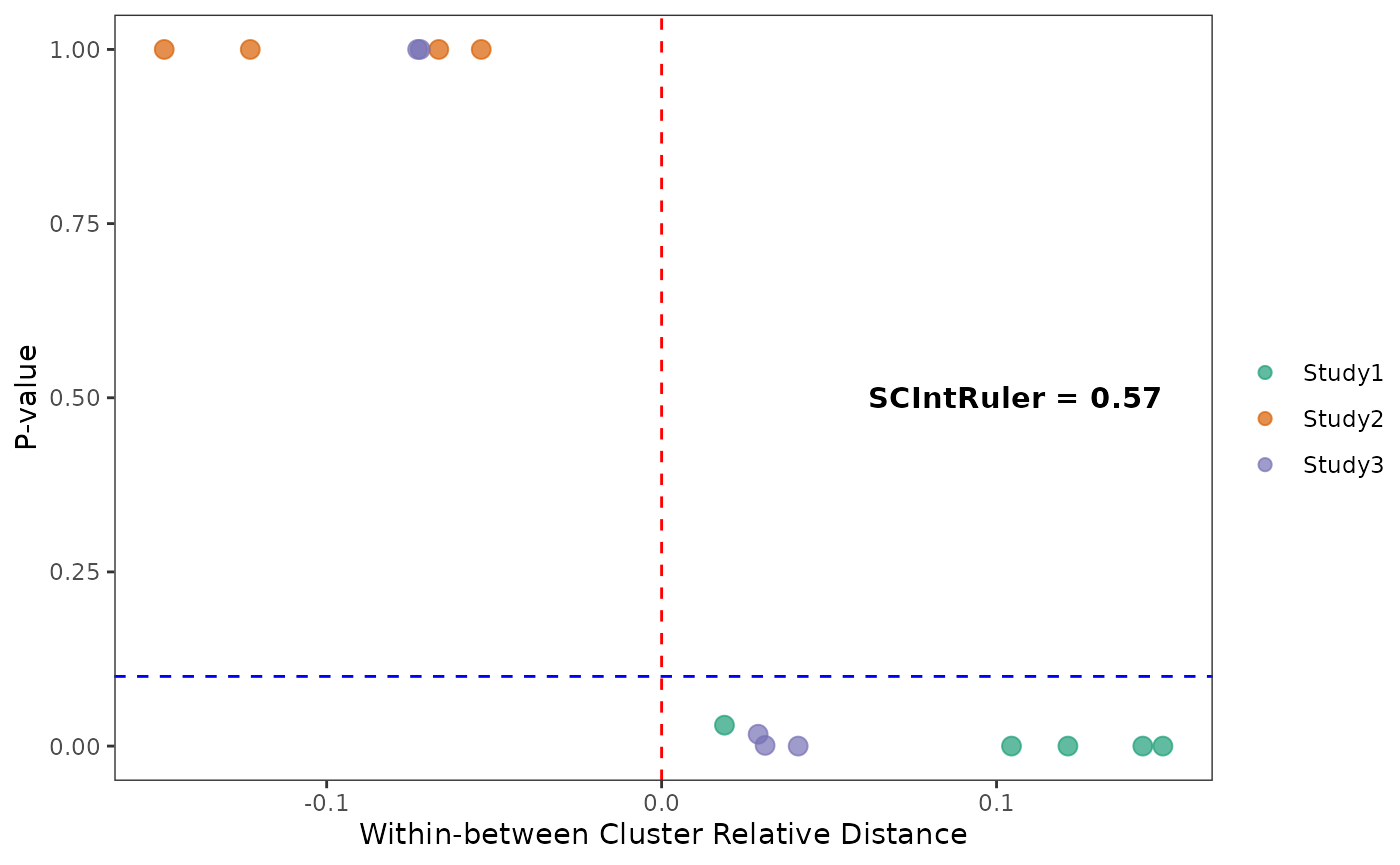
sim_result <- list(fullcluster,normCount,distmat,testres)SessionInfo
#> R version 4.4.1 (2024-06-14)
#> Platform: x86_64-pc-linux-gnu
#> Running under: Ubuntu 24.04.1 LTS
#>
#> Matrix products: default
#> BLAS:   /usr/lib/x86_64-linux-gnu/openblas-pthread/libblas.so.3
#> LAPACK: /usr/lib/x86_64-linux-gnu/openblas-pthread/libopenblasp-r0.3.26.so;  LAPACK version 3.12.0
#>
#> locale:
#>  [1] LC_CTYPE=C.UTF-8       LC_NUMERIC=C           LC_TIME=C.UTF-8
#>  [4] LC_COLLATE=C.UTF-8     LC_MONETARY=C.UTF-8    LC_MESSAGES=C.UTF-8
#>  [7] LC_PAPER=C.UTF-8       LC_NAME=C              LC_ADDRESS=C
#> [10] LC_TELEPHONE=C         LC_MEASUREMENT=C.UTF-8 LC_IDENTIFICATION=C
#>
#> time zone: UTC
#> tzcode source: system (glibc)
#>
#> attached base packages:
#> [1] stats     graphics  grDevices utils     datasets  methods   base
#>
#> other attached packages:
#> [1] ggplot2_3.5.1      dplyr_1.1.4        Seurat_5.1.0       SeuratObject_5.0.2
#> [5] sp_2.1-4           SCIntRuler_0.99.3  BiocStyle_2.32.1
#>
#> loaded via a namespace (and not attached):
#>   [1] RcppAnnoy_0.0.22            splines_4.4.1
#>   [3] later_1.3.2                 batchelor_1.20.0
#>   [5] tibble_3.2.1                polyclip_1.10-7
#>   [7] fastDummies_1.7.4           lifecycle_1.0.4
#>   [9] globals_0.16.3              lattice_0.22-6
#>  [11] MASS_7.3-60.2               magrittr_2.0.3
#>  [13] plotly_4.10.4               sass_0.4.9
#>  [15] rmarkdown_2.28              jquerylib_0.1.4
#>  [17] yaml_2.3.10                 httpuv_1.6.15
#>  [19] sctransform_0.4.1           spam_2.11-0
#>  [21] spatstat.sparse_3.1-0       reticulate_1.39.0
#>  [23] cowplot_1.1.3               pbapply_1.7-2
#>  [25] RColorBrewer_1.1-3          ResidualMatrix_1.14.1
#>  [27] multcomp_1.4-26             abind_1.4-8
#>  [29] zlibbioc_1.50.0             Rtsne_0.17
#>  [31] GenomicRanges_1.56.2        purrr_1.0.2
#>  [33] BiocGenerics_0.50.0         TH.data_1.1-2
#>  [35] sandwich_3.1-1              GenomeInfoDbData_1.2.12
#>  [37] IRanges_2.38.1              S4Vectors_0.42.1
#>  [39] ggrepel_0.9.6               irlba_2.3.5.1
#>  [41] listenv_0.9.1               spatstat.utils_3.1-0
#>  [43] goftest_1.2-3               RSpectra_0.16-2
#>  [45] spatstat.random_3.3-2       fitdistrplus_1.2-1
#>  [47] parallelly_1.38.0           DelayedMatrixStats_1.26.0
#>  [49] pkgdown_2.1.1               coin_1.4-3
#>  [51] leiden_0.4.3.1              codetools_0.2-20
#>  [53] DelayedArray_0.30.1         scuttle_1.14.0
#>  [55] tidyselect_1.2.1            UCSC.utils_1.0.0
#>  [57] farver_2.1.2                ScaledMatrix_1.12.0
#>  [59] matrixStats_1.4.1           stats4_4.4.1
#>  [61] spatstat.explore_3.3-2      jsonlite_1.8.9
#>  [63] BiocNeighbors_1.22.0        progressr_0.14.0
#>  [65] ggridges_0.5.6              survival_3.6-4
#>  [67] systemfonts_1.1.0           tools_4.4.1
#>  [69] ragg_1.3.3                  ica_1.0-3
#>  [71] Rcpp_1.0.13                 glue_1.8.0
#>  [73] gridExtra_2.3               SparseArray_1.4.8
#>  [75] xfun_0.48                   MatrixGenerics_1.16.0
#>  [77] GenomeInfoDb_1.40.1         withr_3.0.1
#>  [79] BiocManager_1.30.25         fastmap_1.2.0
#>  [81] fansi_1.0.6                 digest_0.6.37
#>  [83] rsvd_1.0.5                  R6_2.5.1
#>  [85] mime_0.12                   textshaping_0.4.0
#>  [87] colorspace_2.1-1            scattermore_1.2
#>  [89] tensor_1.5                  spatstat.data_3.1-2
#>  [91] RhpcBLASctl_0.23-42         utf8_1.2.4
#>  [93] tidyr_1.3.1                 generics_0.1.3
#>  [95] data.table_1.16.2           httr_1.4.7
#>  [97] htmlwidgets_1.6.4           S4Arrays_1.4.1
#>  [99] uwot_0.2.2                  pkgconfig_2.0.3
#> [101] gtable_0.3.5                modeltools_0.2-23
#> [103] lmtest_0.9-40               SingleCellExperiment_1.26.0
#> [105] XVector_0.44.0              htmltools_0.5.8.1
#> [107] dotCall64_1.2               bookdown_0.40
#> [109] scales_1.3.0                Biobase_2.64.0
#> [111] png_0.1-8                   harmony_1.2.1
#> [113] spatstat.univar_3.0-1       knitr_1.48
#> [115] reshape2_1.4.4              nlme_3.1-164
#> [117] cachem_1.1.0                zoo_1.8-12
#> [119] stringr_1.5.1               KernSmooth_2.23-24
#> [121] libcoin_1.0-10              parallel_4.4.1
#> [123] miniUI_0.1.1.1              desc_1.4.3
#> [125] pillar_1.9.0                grid_4.4.1
#> [127] vctrs_0.6.5                 RANN_2.6.2
#> [129] promises_1.3.0              BiocSingular_1.20.0
#> [131] beachmat_2.20.0             xtable_1.8-4
#> [133] cluster_2.1.6               evaluate_1.0.1
#> [135] mvtnorm_1.3-1               cli_3.6.3
#> [137] compiler_4.4.1              rlang_1.1.4
#> [139] crayon_1.5.3                future.apply_1.11.2
#> [141] labeling_0.4.3              plyr_1.8.9
#> [143] fs_1.6.4                    stringi_1.8.4
#> [145] viridisLite_0.4.2           deldir_2.0-4
#> [147] BiocParallel_1.38.0         munsell_0.5.1
#> [149] lazyeval_0.2.2              spatstat.geom_3.3-3
#> [151] Matrix_1.7-0                RcppHNSW_0.6.0
#> [153] patchwork_1.3.0             sparseMatrixStats_1.16.0
#> [155] future_1.34.0               shiny_1.9.1
#> [157] SummarizedExperiment_1.34.0 highr_0.11
#> [159] ROCR_1.0-11                 igraph_2.0.3
#> [161] bslib_0.8.0