Dask Array Support to AnnData (original) (raw)
Dask Array Support to AnnData#
Author: Selman Özleyen
Initalizing#
First let’s do our imports and initalize adata objects with the help of the adata_with_dask function defined below.
import dask import dask.array as da import numpy as np import pandas as pd import anndata as ad
dask.config.set({"visualization.engine": "graphviz"});
def adata_with_dask(M, N): adata_dict = {} adata_dict["X"] = da.random.random((M, N)) adata_dict["dtype"] = np.float64 adata_dict["obsm"] = dict( a=da.random.random((M, 100)), ) adata_dict["layers"] = dict( a=da.random.random((M, N)), ) adata_dict["obs"] = pd.DataFrame( {"batch": np.random.choice(["a", "b"], M)}, index=[f"cell{i:03d}" for i in range(M)], ) adata_dict["var"] = pd.DataFrame(index=[f"gene{i:03d}" for i in range(N)])
return ad.AnnData(**adata_dict)Here is how our adata looks like
adata = adata_with_dask(8192,8192) adata
AnnData object with n_obs × n_vars = 8192 × 8192 obs: 'batch' obsm: 'a' layers: 'a'
Representation of Dask Arrays#
Dask arrays consists of chunks that can be distributed in clusters. In the figure below, each small square represents a chunk that form a dask array. In principle these some of these chunks could be in different machines (clusters).
| Array Chunk Bytes 512.00 MiB 128.00 MiB Shape (8192, 8192) (4096, 4096) Dask graph 4 chunks in 1 graph layer Data type float64 numpy.ndarray | 8192 8192 |
|---|
| Array Chunk Bytes 6.25 MiB 6.25 MiB Shape (8192, 100) (8192, 100) Dask graph 1 chunks in 1 graph layer Data type float64 numpy.ndarray | 100 8192 |
|---|
The Computation Graph#
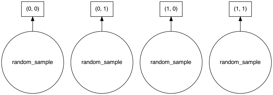
The graph layer in the Count row refers to the layer of the computation graph of the chunks, i.e. which operations are applied to them. We have this because the operations done on Dask arrays aren’t computed instantly. This way, Dask array can optimize the queries we issued to it. It also won’t keep our resources occupied for the results we expect later. Below is a representation of the chunks we initially created.

We now show an example for this computation graph on dask arrays to understand it better. This part is not technically relevant to AnnData.
xsum = adata.X.sum(axis=1) # do a sum on axis=1 xsum
| Array Chunk Bytes 64.00 kiB 32.00 kiB Shape (8192,) (4096,) Dask graph 2 chunks in 3 graph layers Data type float64 numpy.ndarray | 8192 1 |
|---|
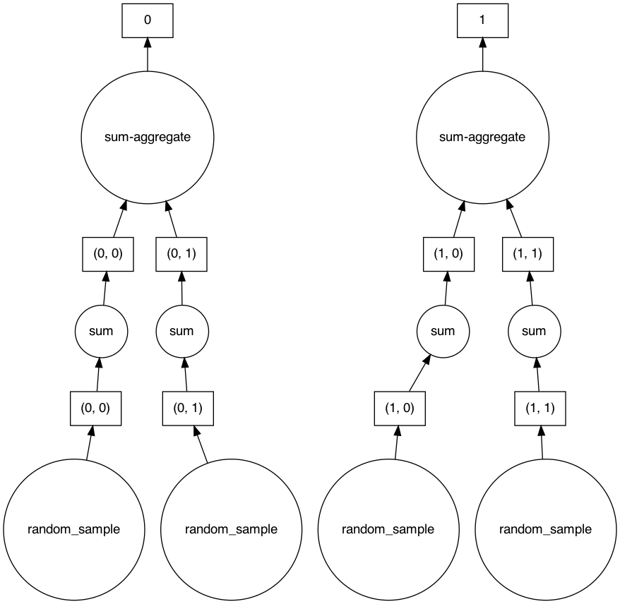
Note that this computation isn’t necessarily done yet, but rather saved to actually run it later. If we investigate the computation graph of this result, we can see that for this operation some chunks aren’t dependent on each other. This might give a hint to the Dask framework to store the chunks that depend on each other to the same cluster. For this simple exercise, all the chunks can be stored in one machine, but when it is impossible to store all the chunks into one machine this will come in handy.

But coming back to our anndata tutorial we will see that nothing changed in our adata.

Concatenation#
In this section we will cover how concatenation on anndata objects that use Dask arrays looks like. We first create another anndata object to concatenate with.
adata2 = adata_with_dask(8192,8192) adata2
AnnData object with n_obs × n_vars = 8192 × 8192 obs: 'batch' obsm: 'a' layers: 'a'
We can see that the X attribute of adata also consist of four chunks.
| Array Chunk Bytes 512.00 MiB 128.00 MiB Shape (8192, 8192) (4096, 4096) Dask graph 4 chunks in 1 graph layer Data type float64 numpy.ndarray | 8192 8192 |
|---|
adata_concat = ad.concat([adata,adata2],index_unique='id')
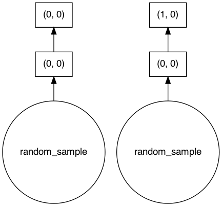
When we concatenate the whole object you can see that in the X of the result consists of eight chunks and they quite probably are just the source chunks aligned.
| Array Chunk Bytes 1.00 GiB 128.00 MiB Shape (16384, 8192) (4096, 4096) Dask graph 8 chunks in 3 graph layers Data type float64 numpy.ndarray | 8192 16384 |
|---|
To confirm this we look at the computation graph. We can confirm that this new object’s X is just the chunks of source X’s put together.
adata_concat.X.visualize()

Here for the obsm we also this. The chunk from both are just stacked on top.
| Array Chunk Bytes 12.50 MiB 6.25 MiB Shape (16384, 100) (8192, 100) Dask graph 2 chunks in 3 graph layers Data type float64 numpy.ndarray | 100 16384 |
|---|
adata_concat.obsm['a'].visualize()

Views#
Let’s see how our views of anndata objects play with Dask arrays.
Slice View#
We take a slice of the concatenated adatas. This operation returns a view of the adata which means that the resulting adata holds a view of the source adata’s Dask array, namely the DaskArrayView class, which is a completely different object than Dask array.
adata_slice_view = adata_concat[:500, :][:, :500]
Below, you can see the values of the X attribute of the result. Which implies that the resulting object isn’t “lazy” like Dask arrays.
| Array Chunk Bytes 1.91 MiB 1.91 MiB Shape (500, 500) (500, 500) Dask graph 1 chunks in 4 graph layers Data type float64 numpy.ndarray | 500 500 |
|---|
But our original adata remains unchanged.
| Array Chunk Bytes 1.00 GiB 128.00 MiB Shape (16384, 8192) (4096, 4096) Dask graph 8 chunks in 3 graph layers Data type float64 numpy.ndarray | 8192 16384 |
|---|
Index List View#
small_view = adata_concat[[12,12,3,5,53],[1,2,5]] small_view
View of AnnData object with n_obs × n_vars = 5 × 3 obs: 'batch' obsm: 'a' layers: 'a'
| Array Chunk Bytes 120 B 120 B Shape (5, 3) (5, 3) Dask graph 1 chunks in 5 graph layers Data type float64 numpy.ndarray | 3 5 |
|---|
View by Category#
categ_view = adata_concat[adata_concat.obs['batch'] == 'b']
| Array Chunk Bytes 511.62 MiB 65.50 MiB Shape (8186, 8192) (2096, 4096) Dask graph 8 chunks in 4 graph layers Data type float64 numpy.ndarray | 8192 8186 |
|---|
To Memory#
| Array Chunk Bytes 1.00 GiB 128.00 MiB Shape (16384, 8192) (4096, 4096) Dask graph 8 chunks in 3 graph layers Data type float64 numpy.ndarray | 8192 16384 |
|---|
Here no copies are made, only the result of the lazy object is asked to be materialized.
adata_mem = adata_concat.to_memory(copy=False) adata_mem.X
array([[0.81114836, 0.6155681 , 0.71416891, ..., 0.66920919, 0.33580076, 0.12920279], [0.00671454, 0.97405959, 0.82439798, ..., 0.13954503, 0.17895137, 0.79356977], [0.38870666, 0.47573504, 0.72575821, ..., 0.96240919, 0.60595132, 0.22621635], ..., [0.34446286, 0.36435086, 0.56605972, ..., 0.72517602, 0.79974538, 0.89232576], [0.19953605, 0.78688055, 0.66993415, ..., 0.73216844, 0.14588037, 0.28056473], [0.48233576, 0.07140058, 0.73679539, ..., 0.9402766 , 0.98517065, 0.41486173]])
If you want to both materialize the result and copy.
adata_mem = adata_concat.to_memory(copy=True) adata_mem.X
array([[0.81114836, 0.6155681 , 0.71416891, ..., 0.66920919, 0.33580076, 0.12920279], [0.00671454, 0.97405959, 0.82439798, ..., 0.13954503, 0.17895137, 0.79356977], [0.38870666, 0.47573504, 0.72575821, ..., 0.96240919, 0.60595132, 0.22621635], ..., [0.34446286, 0.36435086, 0.56605972, ..., 0.72517602, 0.79974538, 0.89232576], [0.19953605, 0.78688055, 0.66993415, ..., 0.73216844, 0.14588037, 0.28056473], [0.48233576, 0.07140058, 0.73679539, ..., 0.9402766 , 0.98517065, 0.41486173]])
IO operations#
Read/Write operations on h5ad and Zarr are supported. One should note that the lazy objects are materialized when this is called. For now, the anndata loaded from file won’t be loaded with dask arrays in it.
Write h5ad#
adata = adata_with_dask(100,100)
adata.write_h5ad('a1.h5ad')
| Array Chunk Bytes 78.12 kiB 78.12 kiB Shape (100, 100) (100, 100) Dask graph 1 chunks in 1 graph layer Data type float64 numpy.ndarray | 100 100 |
|---|
Read h5ad#
h5ad_adata = ad.read_h5ad('a1.h5ad')
array([[0.94530803, 0.5603623 , 0.88396408, ..., 0.5849379 , 0.83891198, 0.47558545], [0.15451784, 0.02692963, 0.9621184 , ..., 0.74202933, 0.21178086, 0.04160213], [0.89403029, 0.81384801, 0.82572102, ..., 0.6824308 , 0.56349224, 0.28945738], ..., [0.13949498, 0.03908582, 0.07293669, ..., 0.35253434, 0.67779358, 0.33458721], [0.56197331, 0.69960036, 0.28042814, ..., 0.44178619, 0.55637234, 0.22577015], [0.53397526, 0.36173157, 0.04517696, ..., 0.67863092, 0.1851758 , 0.43036704]])
Write zarr#
adata.write_zarr('a2.zarr')
| Array Chunk Bytes 78.12 kiB 78.12 kiB Shape (100, 100) (100, 100) Dask graph 1 chunks in 1 graph layer Data type float64 numpy.ndarray | 100 100 |
|---|
Read zarr#
zarr_adata = ad.read_zarr('a2.zarr')
array([[0.94530803, 0.5603623 , 0.88396408, ..., 0.5849379 , 0.83891198, 0.47558545], [0.15451784, 0.02692963, 0.9621184 , ..., 0.74202933, 0.21178086, 0.04160213], [0.89403029, 0.81384801, 0.82572102, ..., 0.6824308 , 0.56349224, 0.28945738], ..., [0.13949498, 0.03908582, 0.07293669, ..., 0.35253434, 0.67779358, 0.33458721], [0.56197331, 0.69960036, 0.28042814, ..., 0.44178619, 0.55637234, 0.22577015], [0.53397526, 0.36173157, 0.04517696, ..., 0.67863092, 0.1851758 , 0.43036704]])
Notice how they are loaded as arrays rather than dask arrays.
Dask Array Support for Other Fields#
This is the list of operations and in which fields they are supported, although some might have not been covered in this tutorial.
The following work with operations anndata supported before are also supported now with Dask arrays:
- anndata.concat()
- Views
- copy()
- to_memory() (changed behaviour)
- read/write on h5ad/zarr
X, obsm, varm, obsp, varp, layers, uns, and raw attributes are all supported and tested.
Note: scipy.sparse array wrapped with dask array doesn’t play well. This is mainly because of the inconsistent numpy api support of scipy.sparse. Even though not explicitly tested, a sparse array that supports the numpy api should theoretically work well.