numpy.random.vonmises — NumPy v1.15 Manual (original) (raw)
numpy.random. vonmises(mu, kappa, size=None)
Draw samples from a von Mises distribution.
Samples are drawn from a von Mises distribution with specified mode (mu) and dispersion (kappa), on the interval [-pi, pi].
The von Mises distribution (also known as the circular normal distribution) is a continuous probability distribution on the unit circle. It may be thought of as the circular analogue of the normal distribution.
| Parameters: | mu : float or array_like of floats Mode (“center”) of the distribution. kappa : float or array_like of floats Dispersion of the distribution, has to be >=0. size : int or tuple of ints, optional Output shape. If the given shape is, e.g., (m, n, k), thenm * n * k samples are drawn. If size is None (default), a single value is returned if mu and kappa are both scalars. Otherwise, np.broadcast(mu, kappa).size samples are drawn. |
|---|---|
| Returns: | out : ndarray or scalar Drawn samples from the parameterized von Mises distribution. |
See also
probability density function, distribution, or cumulative density function, etc.
Notes
The probability density for the von Mises distribution is
p(x) = \frac{e^{\kappa cos(x-\mu)}}{2\pi I_0(\kappa)},
where \mu is the mode and \kappa the dispersion, and I_0(\kappa) is the modified Bessel function of order 0.
The von Mises is named for Richard Edler von Mises, who was born in Austria-Hungary, in what is now the Ukraine. He fled to the United States in 1939 and became a professor at Harvard. He worked in probability theory, aerodynamics, fluid mechanics, and philosophy of science.
References
| [1] | Abramowitz, M. and Stegun, I. A. (Eds.). “Handbook of Mathematical Functions with Formulas, Graphs, and Mathematical Tables, 9th printing,” New York: Dover, 1972. |
|---|
| [2] | von Mises, R., “Mathematical Theory of Probability and Statistics”, New York: Academic Press, 1964. |
|---|
Examples
Draw samples from the distribution:
mu, kappa = 0.0, 4.0 # mean and dispersion s = np.random.vonmises(mu, kappa, 1000)
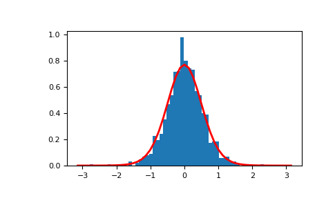
Display the histogram of the samples, along with the probability density function:
import matplotlib.pyplot as plt from scipy.special import i0 plt.hist(s, 50, density=True) x = np.linspace(-np.pi, np.pi, num=51) y = np.exp(kappanp.cos(x-mu))/(2np.pi*i0(kappa)) plt.plot(x, y, linewidth=2, color='r') plt.show()