numpy.random.zipf — NumPy v1.15 Manual (original) (raw)
numpy.random. zipf(a, size=None)
Draw samples from a Zipf distribution.
Samples are drawn from a Zipf distribution with specified parameter_a_ > 1.
The Zipf distribution (also known as the zeta distribution) is a continuous probability distribution that satisfies Zipf’s law: the frequency of an item is inversely proportional to its rank in a frequency table.
| Parameters: | a : float or array_like of floats Distribution parameter. Should be greater than 1. size : int or tuple of ints, optional Output shape. If the given shape is, e.g., (m, n, k), thenm * n * k samples are drawn. If size is None (default), a single value is returned if a is a scalar. Otherwise,np.array(a).size samples are drawn. |
|---|---|
| Returns: | out : ndarray or scalar Drawn samples from the parameterized Zipf distribution. |
See also
probability density function, distribution, or cumulative density function, etc.
Notes
The probability density for the Zipf distribution is
p(x) = \frac{x^{-a}}{\zeta(a)},
where \zeta is the Riemann Zeta function.
It is named for the American linguist George Kingsley Zipf, who noted that the frequency of any word in a sample of a language is inversely proportional to its rank in the frequency table.
References
| [1] | Zipf, G. K., “Selected Studies of the Principle of Relative Frequency in Language,” Cambridge, MA: Harvard Univ. Press, 1932. |
|---|
Examples
Draw samples from the distribution:
a = 2. # parameter s = np.random.zipf(a, 1000)
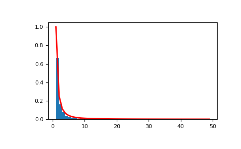
Display the histogram of the samples, along with the probability density function:
import matplotlib.pyplot as plt from scipy import special
Truncate s values at 50 so plot is interesting:
count, bins, ignored = plt.hist(s[s<50], 50, density=True) x = np.arange(1., 50.) y = x**(-a) / special.zetac(a) plt.plot(x, y/max(y), linewidth=2, color='r') plt.show()