numpy.random.noncentral_chisquare — NumPy v1.16 Manual (original) (raw)
numpy.random. noncentral_chisquare(df, nonc, size=None)
Draw samples from a noncentral chi-square distribution.
The noncentral  distribution is a generalisation of the distribution.
| Parameters: | df : float or array_like of floats Degrees of freedom, should be > 0. Changed in version 1.10.0: Earlier NumPy versions required dfnum > 1. nonc : float or array_like of floats Non-centrality, should be non-negative. size : int or tuple of ints, optional Output shape. If the given shape is, e.g., (m, n, k), thenm * n * k samples are drawn. If size is None (default), a single value is returned if df and nonc are both scalars. Otherwise, np.broadcast(df, nonc).size samples are drawn. |
|---|---|
| Returns: | out : ndarray or scalar Drawn samples from the parameterized noncentral chi-square distribution. |
Notes
The probability density function for the noncentral Chi-square distribution is

where  is the Chi-square with q degrees of freedom.
In Delhi (2007), it is noted that the noncentral chi-square is useful in bombing and coverage problems, the probability of killing the point target given by the noncentral chi-squared distribution.
References
| [1] | Delhi, M.S. Holla, “On a noncentral chi-square distribution in the analysis of weapon systems effectiveness”, Metrika, Volume 15, Number 1 / December, 1970. |
|---|
| [2] | Wikipedia, “Noncentral chi-squared distribution”https://en.wikipedia.org/wiki/Noncentral_chi-squared_distribution |
|---|
Examples
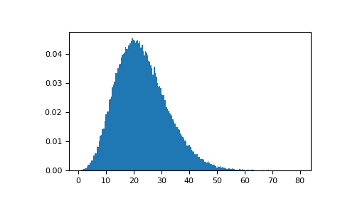
Draw values from the distribution and plot the histogram
import matplotlib.pyplot as plt values = plt.hist(np.random.noncentral_chisquare(3, 20, 100000), ... bins=200, density=True) plt.show()
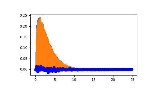
Draw values from a noncentral chisquare with very small noncentrality, and compare to a chisquare.
plt.figure() values = plt.hist(np.random.noncentral_chisquare(3, .0000001, 100000), ... bins=np.arange(0., 25, .1), density=True) values2 = plt.hist(np.random.chisquare(3, 100000), ... bins=np.arange(0., 25, .1), density=True) plt.plot(values[1][0:-1], values[0]-values2[0], 'ob') plt.show()
Demonstrate how large values of non-centrality lead to a more symmetric distribution.
plt.figure() values = plt.hist(np.random.noncentral_chisquare(3, 20, 100000), ... bins=200, density=True) plt.show()
