numpy.random.triangular — NumPy v1.16 Manual (original) (raw)

numpy.random. triangular(left, mode, right, size=None)

Draw samples from the triangular distribution over the interval [left, right].

The triangular distribution is a continuous probability distribution with lower limit left, peak at mode, and upper limit right. Unlike the other distributions, these parameters directly define the shape of the pdf.

Parameters: left : float or array_like of floats Lower limit. mode : float or array_like of floats The value where the peak of the distribution occurs. The value should fulfill the condition left <= mode <= right. right : float or array_like of floats Upper limit, should be larger than left. size : int or tuple of ints, optional Output shape. If the given shape is, e.g., (m, n, k), thenm * n * k samples are drawn. If size is None (default), a single value is returned if left, mode, and rightare all scalars. Otherwise, np.broadcast(left, mode, right).sizesamples are drawn.
Returns: out : ndarray or scalar Drawn samples from the parameterized triangular distribution.

Notes

The probability density function for the triangular distribution is

P(x;l, m, r) = \begin{cases}
\frac{2(x-l)}{(r-l)(m-l)}& \text{for <span class="katex"><span class="katex-mathml"><math xmlns="http://www.w3.org/1998/Math/MathML"><semantics><mrow><mi>l</mi><mo>≤</mo><mi>x</mi><mo>≤</mo><mi>m</mi></mrow><annotation encoding="application/x-tex">l \leq x \leq m</annotation></semantics></math></span><span class="katex-html" aria-hidden="true"><span class="base"><span class="strut" style="height:0.8304em;vertical-align:-0.136em;"></span><span class="mord mathnormal" style="margin-right:0.01968em;">l</span><span class="mspace" style="margin-right:0.2778em;"></span><span class="mrel">≤</span><span class="mspace" style="margin-right:0.2778em;"></span></span><span class="base"><span class="strut" style="height:0.7719em;vertical-align:-0.136em;"></span><span class="mord mathnormal">x</span><span class="mspace" style="margin-right:0.2778em;"></span><span class="mrel">≤</span><span class="mspace" style="margin-right:0.2778em;"></span></span><span class="base"><span class="strut" style="height:0.4306em;"></span><span class="mord mathnormal">m</span></span></span></span>},\\
\frac{2(r-x)}{(r-l)(r-m)}& \text{for <span class="katex"><span class="katex-mathml"><math xmlns="http://www.w3.org/1998/Math/MathML"><semantics><mrow><mi>m</mi><mo>≤</mo><mi>x</mi><mo>≤</mo><mi>r</mi></mrow><annotation encoding="application/x-tex">m \leq x \leq r</annotation></semantics></math></span><span class="katex-html" aria-hidden="true"><span class="base"><span class="strut" style="height:0.7719em;vertical-align:-0.136em;"></span><span class="mord mathnormal">m</span><span class="mspace" style="margin-right:0.2778em;"></span><span class="mrel">≤</span><span class="mspace" style="margin-right:0.2778em;"></span></span><span class="base"><span class="strut" style="height:0.7719em;vertical-align:-0.136em;"></span><span class="mord mathnormal">x</span><span class="mspace" style="margin-right:0.2778em;"></span><span class="mrel">≤</span><span class="mspace" style="margin-right:0.2778em;"></span></span><span class="base"><span class="strut" style="height:0.4306em;"></span><span class="mord mathnormal" style="margin-right:0.02778em;">r</span></span></span></span>},\\
0& \text{otherwise}.
\end{cases}

The triangular distribution is often used in ill-defined problems where the underlying distribution is not known, but some knowledge of the limits and mode exists. Often it is used in simulations.

References

[1] Wikipedia, “Triangular distribution”https://en.wikipedia.org/wiki/Triangular_distribution

Examples

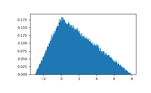
Draw values from the distribution and plot the histogram:

import matplotlib.pyplot as plt h = plt.hist(np.random.triangular(-3, 0, 8, 100000), bins=200, ... density=True) plt.show()

../../_images/numpy-random-triangular-1.png