BSpline — SciPy v1.15.3 Manual (original) (raw)
scipy.interpolate.
class scipy.interpolate.BSpline(t, c, k, extrapolate=True, axis=0)[source]#
Univariate spline in the B-spline basis.
\[S(x) = \sum_{j=0}^{n-1} c_j B_{j, k; t}(x)\]
where \(B_{j, k; t}\) are B-spline basis functions of degree _k_and knots t.
Parameters:
tndarray, shape (n+k+1,)
knots
cndarray, shape (>=n, …)
spline coefficients
kint
B-spline degree
extrapolatebool or ‘periodic’, optional
whether to extrapolate beyond the base interval, t[k] .. t[n], or to return nans. If True, extrapolates the first and last polynomial pieces of b-spline functions active on the base interval. If ‘periodic’, periodic extrapolation is used. Default is True.
axisint, optional
Interpolation axis. Default is zero.
Notes
B-spline basis elements are defined via
\[ \begin{align}\begin{aligned}B_{i, 0}(x) = 1, \textrm{if tilex<ti+1t_i \le x < t_{i+1}tilex<ti+1, otherwise 000,}\\B_{i, k}(x) = \frac{x - t_i}{t_{i+k} - t_i} B_{i, k-1}(x) + \frac{t_{i+k+1} - x}{t_{i+k+1} - t_{i+1}} B_{i+1, k-1}(x)\end{aligned}\end{align} \]
Implementation details
- At least
k+1coefficients are required for a spline of degree k, so thatn >= k+1. Additional coefficients,c[j]withj > n, are ignored. - B-spline basis elements of degree k form a partition of unity on the_base interval_,
t[k] <= x <= t[n].
References
[2]
Carl de Boor, A practical guide to splines, Springer, 2001.
Examples
Translating the recursive definition of B-splines into Python code, we have:
def B(x, k, i, t): ... if k == 0: ... return 1.0 if t[i] <= x < t[i+1] else 0.0 ... if t[i+k] == t[i]: ... c1 = 0.0 ... else: ... c1 = (x - t[i])/(t[i+k] - t[i]) * B(x, k-1, i, t) ... if t[i+k+1] == t[i+1]: ... c2 = 0.0 ... else: ... c2 = (t[i+k+1] - x)/(t[i+k+1] - t[i+1]) * B(x, k-1, i+1, t) ... return c1 + c2
def bspline(x, t, c, k): ... n = len(t) - k - 1 ... assert (n >= k+1) and (len(c) >= n) ... return sum(c[i] * B(x, k, i, t) for i in range(n))
Note that this is an inefficient (if straightforward) way to evaluate B-splines — this spline class does it in an equivalent, but much more efficient way.
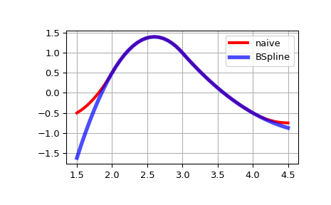
Here we construct a quadratic spline function on the base interval2 <= x <= 4 and compare with the naive way of evaluating the spline:
from scipy.interpolate import BSpline k = 2 t = [0, 1, 2, 3, 4, 5, 6] c = [-1, 2, 0, -1] spl = BSpline(t, c, k) spl(2.5) array(1.375) bspline(2.5, t, c, k) 1.375
Note that outside of the base interval results differ. This is becauseBSpline extrapolates the first and last polynomial pieces of B-spline functions active on the base interval.
import matplotlib.pyplot as plt import numpy as np fig, ax = plt.subplots() xx = np.linspace(1.5, 4.5, 50) ax.plot(xx, [bspline(x, t, c ,k) for x in xx], 'r-', lw=3, label='naive') ax.plot(xx, spl(xx), 'b-', lw=4, alpha=0.7, label='BSpline') ax.grid(True) ax.legend(loc='best') plt.show()
Attributes:
tndarray
knot vector
cndarray
spline coefficients
kint
spline degree
extrapolatebool
If True, extrapolates the first and last polynomial pieces of b-spline functions active on the base interval.
axisint
Interpolation axis.
tcktuple
Equivalent to (self.t, self.c, self.k) (read-only).
Methods
| __call__(x[, nu, extrapolate]) | Evaluate a spline function. |
|---|---|
| basis_element(t[, extrapolate]) | Return a B-spline basis element B(x | t[0], ..., t[k+1]). |
| derivative([nu]) | Return a B-spline representing the derivative. |
| antiderivative([nu]) | Return a B-spline representing the antiderivative. |
| integrate(a, b[, extrapolate]) | Compute a definite integral of the spline. |
| insert_knot(x[, m]) | Insert a new knot at x of multiplicity m. |
| construct_fast(t, c, k[, extrapolate, axis]) | Construct a spline without making checks. |
| design_matrix(x, t, k[, extrapolate]) | Returns a design matrix as a CSR format sparse array. |
| from_power_basis(pp[, bc_type]) | Construct a polynomial in the B-spline basis from a piecewise polynomial in the power basis. |