ev — SciPy v1.15.3 Manual (original) (raw)

scipy.interpolate.BivariateSpline.

BivariateSpline.ev(xi, yi, dx=0, dy=0)[source]#

Evaluate the spline at points

Returns the interpolated value at (xi[i], yi[i]), i=0,...,len(xi)-1.

Parameters:

xi, yiarray_like

Input coordinates. Standard Numpy broadcasting is obeyed. The ordering of axes is consistent withnp.meshgrid(..., indexing="ij") and inconsistent with the default ordering np.meshgrid(..., indexing="xy").

dxint, optional

Order of x-derivative

Added in version 0.14.0.

dyint, optional

Order of y-derivative

Added in version 0.14.0.

Examples

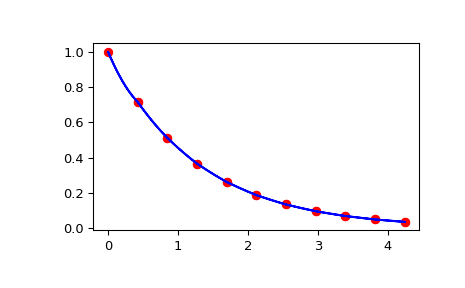
Suppose that we want to bilinearly interpolate an exponentially decaying function in 2 dimensions.

import numpy as np from scipy.interpolate import RectBivariateSpline def f(x, y): ... return np.exp(-np.sqrt((x / 2) ** 2 + y**2))

We sample the function on a coarse grid and set up the interpolator. Note that the default indexing="xy" of meshgrid would result in an unexpected (transposed) result after interpolation.

xarr = np.linspace(-3, 3, 21) yarr = np.linspace(-3, 3, 21) xgrid, ygrid = np.meshgrid(xarr, yarr, indexing="ij") zdata = f(xgrid, ygrid) rbs = RectBivariateSpline(xarr, yarr, zdata, kx=1, ky=1)

Next we sample the function along a diagonal slice through the coordinate space on a finer grid using interpolation.

xinterp = np.linspace(-3, 3, 201) yinterp = np.linspace(3, -3, 201) zinterp = rbs.ev(xinterp, yinterp)

And check that the interpolation passes through the function evaluations as a function of the distance from the origin along the slice.

import matplotlib.pyplot as plt fig = plt.figure() ax1 = fig.add_subplot(1, 1, 1) ax1.plot(np.sqrt(xarr2 + yarr2), np.diag(zdata), "or") ax1.plot(np.sqrt(xinterp2 + yinterp2), zinterp, "-b") plt.show()