SmoothSphereBivariateSpline — SciPy v1.15.2 Manual (original) (raw)

scipy.interpolate.

class scipy.interpolate.SmoothSphereBivariateSpline(theta, phi, r, w=None, s=0.0, eps=1e-16)[source]#

Smooth bivariate spline approximation in spherical coordinates.

Added in version 0.11.0.

Parameters:

theta, phi, rarray_like

1-D sequences of data points (order is not important). Coordinates must be given in radians. Theta must lie within the interval[0, pi], and phi must lie within the interval [0, 2pi].

warray_like, optional

Positive 1-D sequence of weights.

sfloat, optional

Positive smoothing factor defined for estimation condition:sum((w(i)*(r(i) - s(theta(i), phi(i))))**2, axis=0) <= sDefault s=len(w) which should be a good value if 1/w[i] is an estimate of the standard deviation of r[i].

epsfloat, optional

A threshold for determining the effective rank of an over-determined linear system of equations. eps should have a value within the open interval (0, 1), the default is 1e-16.

Notes

For more information, see the FITPACK site about this function.

Examples

Suppose we have global data on a coarse grid (the input data does not have to be on a grid):

import numpy as np theta = np.linspace(0., np.pi, 7) phi = np.linspace(0., 2*np.pi, 9) data = np.empty((theta.shape[0], phi.shape[0])) data[:,0], data[0,:], data[-1,:] = 0., 0., 0. data[1:-1,1], data[1:-1,-1] = 1., 1. data[1,1:-1], data[-2,1:-1] = 1., 1. data[2:-2,2], data[2:-2,-2] = 2., 2. data[2,2:-2], data[-3,2:-2] = 2., 2. data[3,3:-2] = 3. data = np.roll(data, 4, 1)

We need to set up the interpolator object

lats, lons = np.meshgrid(theta, phi) from scipy.interpolate import SmoothSphereBivariateSpline lut = SmoothSphereBivariateSpline(lats.ravel(), lons.ravel(), ... data.T.ravel(), s=3.5)

As a first test, we’ll see what the algorithm returns when run on the input coordinates

data_orig = lut(theta, phi)

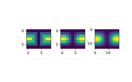
Finally we interpolate the data to a finer grid

fine_lats = np.linspace(0., np.pi, 70) fine_lons = np.linspace(0., 2 * np.pi, 90)

data_smth = lut(fine_lats, fine_lons)

import matplotlib.pyplot as plt fig = plt.figure() ax1 = fig.add_subplot(131) ax1.imshow(data, interpolation='nearest') ax2 = fig.add_subplot(132) ax2.imshow(data_orig, interpolation='nearest') ax3 = fig.add_subplot(133) ax3.imshow(data_smth, interpolation='nearest') plt.show()

Methods