extent — SciPy v1.15.3 Manual (original) (raw)

scipy.signal.ShortTimeFFT.

ShortTimeFFT.extent(n, axes_seq='tf', center_bins=False)[source]#

Return minimum and maximum values time-frequency values.

A tuple with four floats (t0, t1, f0, f1) for ‘tf’ and(f0, f1, t0, t1) for ‘ft’ is returned describing the corners of the time-frequency domain of the stft. That tuple can be passed to matplotlib.pyplot.imshow as a parameter with the same name.

Parameters:

nint

Number of samples in input signal.

axes_seq{‘tf’, ‘ft’}

Return time extent first and then frequency extent or vice-versa.

center_bins: bool

If set (default False), the values of the time slots and frequency bins are moved from the side the middle. This is useful, when plotting the stft values as step functions, i.e., with no interpolation.

Examples

The following two plots illustrate the effect of the parameter center_bins: The grid lines represent the three time and the four frequency values of the STFT. The left plot, where (t0, t1, f0, f1) = (0, 3, 0, 4) is passed as parameterextent to imshow, shows the standard behavior of the time and frequency values being at the lower edge of the corrsponding bin. The right plot, with (t0, t1, f0, f1) = (-0.5, 2.5, -0.5, 3.5), shows that the bins are centered over the respective values when passingcenter_bins=True.

import matplotlib.pyplot as plt import numpy as np from scipy.signal import ShortTimeFFT ... n, m = 12, 6 SFT = ShortTimeFFT.from_window('hann', fs=m, nperseg=m, noverlap=0) Sxx = SFT.stft(np.cos(np.arange(n))) # produces a colorful plot ... fig, axx = plt.subplots(1, 2, tight_layout=True, figsize=(6., 4.)) for ax_, center_bins in zip(axx, (False, True)): ... ax_.imshow(abs(Sxx), origin='lower', interpolation=None, aspect='equal', ... cmap='viridis', extent=SFT.extent(n, 'tf', center_bins)) ... ax_.set_title(f"{center_bins=}") ... ax_.set_xlabel(f"Time ({SFT.p_num(n)} points, Δt={SFT.delta_t})") ... ax_.set_ylabel(f"Frequency ({SFT.f_pts} points, Δf={SFT.delta_f})") ... ax_.set_xticks(SFT.t(n)) # vertical grid line are timestamps ... ax_.set_yticks(SFT.f) # horizontal grid line are frequency values ... ax_.grid(True) plt.show()

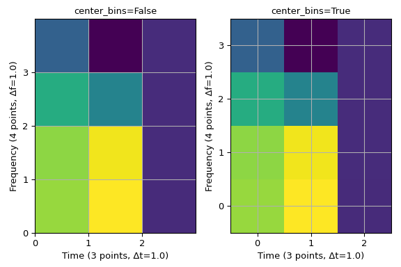
Note that the step-like behavior with the constant colors is caused by passinginterpolation=None to imshow.