bilinear — SciPy v1.16.0 Manual (original) (raw)

scipy.signal.

scipy.signal.bilinear(b, a, fs=1.0)[source]#

Calculate a digital IIR filter from an analog transfer function by utilizing the bilinear transform.

Parameters:

barray_like

Coefficients of the numerator polynomial of the analog transfer function in form of a complex- or real-valued 1d array.

aarray_like

Coefficients of the denominator polynomial of the analog transfer function in form of a complex- or real-valued 1d array.

fsfloat

Sample rate, as ordinary frequency (e.g., hertz). No pre-warping is done in this function.

Returns:

betandarray

Coefficients of the numerator polynomial of the digital transfer function in form of a complex- or real-valued 1d array.

alphandarray

Coefficients of the denominator polynomial of the digital transfer function in form of a complex- or real-valued 1d array.

Notes

The parameters \(b = [b_0, \ldots, b_Q]\) and \(a = [a_0, \ldots, a_P]\)are 1d arrays of length \(Q+1\) and \(P+1\). They define the analog transfer function

\[H_a(s) = \frac{b_0 s^Q + b_1 s^{Q-1} + \cdots + b_Q}{ a_0 s^P + a_1 s^{P-1} + \cdots + a_P}\ .\]

The bilinear transform [1] is applied by substituting

\[s = \kappa \frac{z-1}{z+1}\ , \qquad \kappa := 2 f_s\ ,\]

into \(H_a(s)\), with \(f_s\) being the sampling rate. This results in the digital transfer function in the \(z\)-domain

\[H_d(z) = \frac{b_0 \left(\kappa \frac{z-1}{z+1}\right)^Q + b_1 \left(\kappa \frac{z-1}{z+1}\right)^{Q-1} + \cdots + b_Q}{ a_0 \left(\kappa \frac{z-1}{z+1}\right)^P + a_1 \left(\kappa \frac{z-1}{z+1}\right)^{P-1} + \cdots + a_P}\ .\]

This expression can be simplified by multiplying numerator and denominator by\((z+1)^N\), with \(N=\max(P, Q)\). This allows \(H_d(z)\) to be reformulated as

\[\begin{split}& & \frac{b_0 \big(\kappa (z-1)\big)^Q (z+1)^{N-Q} + b_1 \big(\kappa (z-1)\big)^{Q-1} (z+1)^{N-Q+1} + \cdots + b_Q(z+1)^N}{ a_0 \big(\kappa (z-1)\big)^P (z+1)^{N-P} + a_1 \big(\kappa (z-1)\big)^{P-1} (z+1)^{N-P+1} + \cdots + a_P(z+1)^N}\\ &=:& \frac{\beta_0 + \beta_1 z^{-1} + \cdots + \beta_N z^{-N}}{ \alpha_0 + \alpha_1 z^{-1} + \cdots + \alpha_N z^{-N}}\ .\end{split}\]

This is the equation implemented to perform the bilinear transform. Note that for large \(f_s\), \(\kappa^Q\) or \(\kappa^P\) can cause a numeric overflow for sufficiently large \(P\) or \(Q\).

References

Examples

The following example shows the frequency response of an analog bandpass filter and the corresponding digital filter derived by utilitzing the bilinear transform:

from scipy import signal import matplotlib.pyplot as plt import numpy as np ... fs = 100 # sampling frequency om_c = 2 * np.pi * np.array([7, 13]) # corner frequencies bb_s, aa_s = signal.butter(4, om_c, btype='bandpass', analog=True, output='ba') bb_z, aa_z = signal.bilinear(bb_s, aa_s, fs) ... w_z, H_z = signal.freqz(bb_z, aa_z) # frequency response of digitial filter w_s, H_s = signal.freqs(bb_s, aa_s, worN=w_zfs) # analog filter response ... f_z, f_s = w_z * fs / (2np.pi), w_s / (2np.pi) Hz_dB, Hs_dB = (20np.log10(np.abs(H_).clip(1e-10)) for H_ in (H_z, H_s)) fg0, ax0 = plt.subplots() ax0.set_title("Frequency Response of 4-th order Bandpass Filter") ax0.set(xlabel='Frequency fff in Hertz', ylabel='Magnitude in dB', ... xlim=[f_z[1], fs/2], ylim=[-200, 2]) ax0.semilogx(f_z, Hz_dB, alpha=.5, label=r'$|H_z(e^{j 2 \pi f})|$') ax0.semilogx(f_s, Hs_dB, alpha=.5, label=r'$|H_s(j 2 \pi f)|$') ax0.legend() ax0.grid(which='both', axis='x') ax0.grid(which='major', axis='y') plt.show()

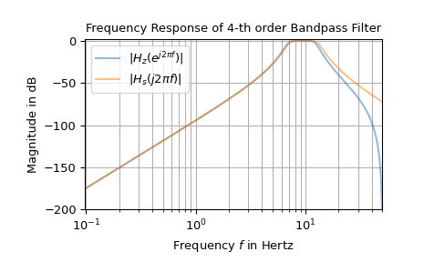
The difference in the higher frequencies shown in the plot is caused by an effect called “frequency warping”. [1] describes a method called “pre-warping” to reduce those deviations.