gausspulse — SciPy v1.15.3 Manual (original) (raw)

scipy.signal.

scipy.signal.gausspulse(t, fc=1000, bw=0.5, bwr=-6, tpr=-60, retquad=False, retenv=False)[source]#

Return a Gaussian modulated sinusoid:

exp(-a t^2) exp(1j*2*pi*fc*t).

If retquad is True, then return the real and imaginary parts (in-phase and quadrature). If retenv is True, then return the envelope (unmodulated signal). Otherwise, return the real part of the modulated sinusoid.

Parameters:

tndarray or the string ‘cutoff’

Input array.

fcfloat, optional

Center frequency (e.g. Hz). Default is 1000.

bwfloat, optional

Fractional bandwidth in frequency domain of pulse (e.g. Hz). Default is 0.5.

bwrfloat, optional

Reference level at which fractional bandwidth is calculated (dB). Default is -6.

tprfloat, optional

If t is ‘cutoff’, then the function returns the cutoff time for when the pulse amplitude falls below tpr (in dB). Default is -60.

retquadbool, optional

If True, return the quadrature (imaginary) as well as the real part of the signal. Default is False.

retenvbool, optional

If True, return the envelope of the signal. Default is False.

Returns:

yIndarray

Real part of signal. Always returned.

yQndarray

Imaginary part of signal. Only returned if retquad is True.

yenvndarray

Envelope of signal. Only returned if retenv is True.

Examples

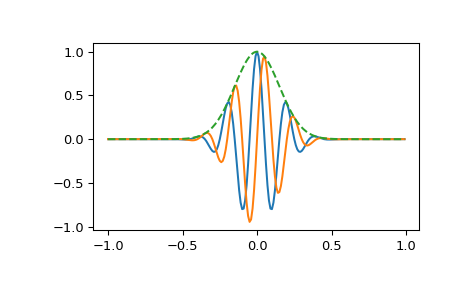
Plot real component, imaginary component, and envelope for a 5 Hz pulse, sampled at 100 Hz for 2 seconds:

import numpy as np from scipy import signal import matplotlib.pyplot as plt t = np.linspace(-1, 1, 2 * 100, endpoint=False) i, q, e = signal.gausspulse(t, fc=5, retquad=True, retenv=True) plt.plot(t, i, t, q, t, e, '--')