iirfilter — SciPy v1.15.3 Manual (original) (raw)

scipy.signal.

scipy.signal.iirfilter(N, Wn, rp=None, rs=None, btype='band', analog=False, ftype='butter', output='ba', fs=None)[source]#

IIR digital and analog filter design given order and critical points.

Design an Nth-order digital or analog filter and return the filter coefficients.

Parameters:

Nint

The order of the filter.

Wnarray_like

A scalar or length-2 sequence giving the critical frequencies.

For digital filters, Wn are in the same units as fs. By default,fs is 2 half-cycles/sample, so these are normalized from 0 to 1, where 1 is the Nyquist frequency. (Wn is thus in half-cycles / sample.)

For analog filters, Wn is an angular frequency (e.g., rad/s).

When Wn is a length-2 sequence, Wn[0] must be less than Wn[1].

rpfloat, optional

For Chebyshev and elliptic filters, provides the maximum ripple in the passband. (dB)

rsfloat, optional

For Chebyshev and elliptic filters, provides the minimum attenuation in the stop band. (dB)

btype{‘bandpass’, ‘lowpass’, ‘highpass’, ‘bandstop’}, optional

The type of filter. Default is ‘bandpass’.

analogbool, optional

When True, return an analog filter, otherwise a digital filter is returned.

ftypestr, optional

The type of IIR filter to design:

• Butterworth : ‘butter’
• Chebyshev I : ‘cheby1’
• Chebyshev II : ‘cheby2’
• Cauer/elliptic: ‘ellip’
• Bessel/Thomson: ‘bessel’

output{‘ba’, ‘zpk’, ‘sos’}, optional

Filter form of the output:

• second-order sections (recommended): ‘sos’
• numerator/denominator (default) : ‘ba’
• pole-zero : ‘zpk’

In general the second-order sections (‘sos’) form is recommended because inferring the coefficients for the numerator/denominator form (‘ba’) suffers from numerical instabilities. For reasons of backward compatibility the default form is the numerator/denominator form (‘ba’), where the ‘b’ and the ‘a’ in ‘ba’ refer to the commonly used names of the coefficients used.

Note: Using the second-order sections form (‘sos’) is sometimes associated with additional computational costs: for data-intense use cases it is therefore recommended to also investigate the numerator/denominator form (‘ba’).

fsfloat, optional

The sampling frequency of the digital system.

Added in version 1.2.0.

Returns:

b, andarray, ndarray

Numerator (b) and denominator (a) polynomials of the IIR filter. Only returned if output='ba'.

z, p, kndarray, ndarray, float

Zeros, poles, and system gain of the IIR filter transfer function. Only returned if output='zpk'.

sosndarray

Second-order sections representation of the IIR filter. Only returned if output='sos'.

Notes

The 'sos' output parameter was added in 0.16.0.

Examples

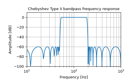
Generate a 17th-order Chebyshev II analog bandpass filter from 50 Hz to 200 Hz and plot the frequency response:

import numpy as np from scipy import signal import matplotlib.pyplot as plt

b, a = signal.iirfilter(17, [2np.pi50, 2np.pi200], rs=60, ... btype='band', analog=True, ftype='cheby2') w, h = signal.freqs(b, a, 1000) fig = plt.figure() ax = fig.add_subplot(1, 1, 1) ax.semilogx(w / (2*np.pi), 20 * np.log10(np.maximum(abs(h), 1e-5))) ax.set_title('Chebyshev Type II bandpass frequency response') ax.set_xlabel('Frequency [Hz]') ax.set_ylabel('Amplitude [dB]') ax.axis((10, 1000, -100, 10)) ax.grid(which='both', axis='both') plt.show()

Create a digital filter with the same properties, in a system with sampling rate of 2000 Hz, and plot the frequency response. (Second-order sections implementation is required to ensure stability of a filter of this order):

sos = signal.iirfilter(17, [50, 200], rs=60, btype='band', ... analog=False, ftype='cheby2', fs=2000, ... output='sos') w, h = signal.freqz_sos(sos, 2000, fs=2000) fig = plt.figure() ax = fig.add_subplot(1, 1, 1) ax.semilogx(w, 20 * np.log10(np.maximum(abs(h), 1e-5))) ax.set_title('Chebyshev Type II bandpass frequency response') ax.set_xlabel('Frequency [Hz]') ax.set_ylabel('Amplitude [dB]') ax.axis((10, 1000, -100, 10)) ax.grid(which='both', axis='both') plt.show()