periodogram — SciPy v1.15.3 Manual (original) (raw)
scipy.signal.
scipy.signal.periodogram(x, fs=1.0, window='boxcar', nfft=None, detrend='constant', return_onesided=True, scaling='density', axis=-1)[source]#
Estimate power spectral density using a periodogram.
Parameters:
xarray_like
Time series of measurement values
fsfloat, optional
Sampling frequency of the x time series. Defaults to 1.0.
windowstr or tuple or array_like, optional
Desired window to use. If window is a string or tuple, it is passed to get_window to generate the window values, which are DFT-even by default. See get_window for a list of windows and required parameters. If window is array_like it will be used directly as the window and its length must be equal to the length of the axis over which the periodogram is computed. Defaults to ‘boxcar’.
nfftint, optional
Length of the FFT used. If None the length of x will be used.
detrendstr or function or False, optional
Specifies how to detrend each segment. If detrend is a string, it is passed as the type argument to the detrendfunction. If it is a function, it takes a segment and returns a detrended segment. If detrend is False, no detrending is done. Defaults to ‘constant’.
return_onesidedbool, optional
If True, return a one-sided spectrum for real data. If_False_ return a two-sided spectrum. Defaults to True, but for complex data, a two-sided spectrum is always returned.
scaling{ ‘density’, ‘spectrum’ }, optional
Selects between computing the power spectral density (‘density’) where Pxx has units of V**2/Hz and computing the squared magnitude spectrum (‘spectrum’) where Pxx has units of V**2, if _x_is measured in V and fs is measured in Hz. Defaults to ‘density’
axisint, optional
Axis along which the periodogram is computed; the default is over the last axis (i.e. axis=-1).
Returns:
fndarray
Array of sample frequencies.
Pxxndarray
Power spectral density or power spectrum of x.
See also
Estimate power spectral density using Welch’s method
Lomb-Scargle periodogram for unevenly sampled data
Notes
Consult the Spectral Analysis section of the SciPy User Guidefor a discussion of the scalings of the power spectral density and the magnitude (squared) spectrum.
Added in version 0.12.0.
Examples
import numpy as np from scipy import signal import matplotlib.pyplot as plt rng = np.random.default_rng()
Generate a test signal, a 2 Vrms sine wave at 1234 Hz, corrupted by 0.001 V**2/Hz of white noise sampled at 10 kHz.
fs = 10e3 N = 1e5 amp = 2np.sqrt(2) freq = 1234.0 noise_power = 0.001 * fs / 2 time = np.arange(N) / fs x = ampnp.sin(2np.pifreq*time) x += rng.normal(scale=np.sqrt(noise_power), size=time.shape)
Compute and plot the power spectral density.
f, Pxx_den = signal.periodogram(x, fs) plt.semilogy(f, Pxx_den) plt.ylim([1e-7, 1e2]) plt.xlabel('frequency [Hz]') plt.ylabel('PSD [V**2/Hz]') plt.show()
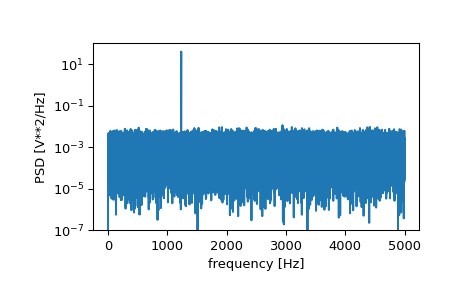
If we average the last half of the spectral density, to exclude the peak, we can recover the noise power on the signal.
np.mean(Pxx_den[25000:]) 0.000985320699252543
Now compute and plot the power spectrum.
f, Pxx_spec = signal.periodogram(x, fs, 'flattop', scaling='spectrum') plt.figure() plt.semilogy(f, np.sqrt(Pxx_spec)) plt.ylim([1e-4, 1e1]) plt.xlabel('frequency [Hz]') plt.ylabel('Linear spectrum [V RMS]') plt.show()
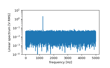
The peak height in the power spectrum is an estimate of the RMS amplitude.
np.sqrt(Pxx_spec.max()) 2.0077340678640727