sweep_poly — SciPy v1.15.3 Manual (original) (raw)

scipy.signal.

scipy.signal.sweep_poly(t, poly, phi=0)[source]#

Frequency-swept cosine generator, with a time-dependent frequency.

This function generates a sinusoidal function whose instantaneous frequency varies with time. The frequency at time t is given by the polynomial poly.

Parameters:

tndarray

Times at which to evaluate the waveform.

poly1-D array_like or instance of numpy.poly1d

The desired frequency expressed as a polynomial. If poly is a list or ndarray of length n, then the elements of poly are the coefficients of the polynomial, and the instantaneous frequency is

f(t) = poly[0]*t**(n-1) + poly[1]*t**(n-2) + ... + poly[n-1]

If poly is an instance of numpy.poly1d, then the instantaneous frequency is

f(t) = poly(t)

phifloat, optional

Phase offset, in degrees, Default: 0.

Returns:

sweep_polyndarray

A numpy array containing the signal evaluated at t with the requested time-varying frequency. More precisely, the function returns cos(phase + (pi/180)*phi), where phase is the integral (from 0 to t) of 2 * pi * f(t); f(t) is defined above.

Notes

Added in version 0.8.0.

If poly is a list or ndarray of length n, then the elements of_poly_ are the coefficients of the polynomial, and the instantaneous frequency is:

f(t) = poly[0]*t**(n-1) + poly[1]*t**(n-2) + ... + poly[n-1]

If poly is an instance of numpy.poly1d, then the instantaneous frequency is:

f(t) = poly(t)

Finally, the output s is:

cos(phase + (pi/180)*phi)

where phase is the integral from 0 to t of 2 * pi * f(t),f(t) as defined above.

Examples

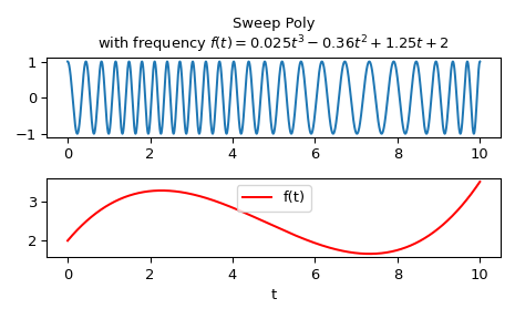
Compute the waveform with instantaneous frequency:

f(t) = 0.025t**3 - 0.36t*2 + 1.25t + 2

over the interval 0 <= t <= 10.

import numpy as np from scipy.signal import sweep_poly p = np.poly1d([0.025, -0.36, 1.25, 2.0]) t = np.linspace(0, 10, 5001) w = sweep_poly(t, p)

Plot it:

import matplotlib.pyplot as plt plt.subplot(2, 1, 1) plt.plot(t, w) plt.title("Sweep Poly\nwith frequency " + ... "$f(t) = 0.025t^3 - 0.36t^2 + 1.25t + 2$") plt.subplot(2, 1, 2) plt.plot(t, p(t), 'r', label='f(t)') plt.legend() plt.xlabel('t') plt.tight_layout() plt.show()