zoom_fft — SciPy v1.15.3 Manual (original) (raw)
scipy.signal.
scipy.signal.zoom_fft(x, fn, m=None, *, fs=2, endpoint=False, axis=-1)[source]#
Compute the DFT of x only for frequencies in range fn.
Parameters:
xarray
The signal to transform.
fnarray_like
A length-2 sequence [f1, _f2_] giving the frequency range, or a scalar, for which the range [0, _fn_] is assumed.
mint, optional
The number of points to evaluate. The default is the length of x.
fsfloat, optional
The sampling frequency. If fs=10 represented 10 kHz, for example, then f1 and f2 would also be given in kHz. The default sampling frequency is 2, so f1 and f2 should be in the range [0, 1] to keep the transform below the Nyquist frequency.
endpointbool, optional
If True, f2 is the last sample. Otherwise, it is not included. Default is False.
axisint, optional
Axis over which to compute the FFT. If not given, the last axis is used.
Returns:
outndarray
The transformed signal. The Fourier transform will be calculated at the points f1, f1+df, f1+2df, …, f2, where df=(f2-f1)/m.
See also
Class that creates a callable partial FFT function.
Notes
The defaults are chosen such that signal.zoom_fft(x, 2) is equivalent to fft.fft(x) and, if m > len(x), that signal.zoom_fft(x, 2, m)is equivalent to fft.fft(x, m).
To graph the magnitude of the resulting transform, use:
plot(linspace(f1, f2, m, endpoint=False), abs(zoom_fft(x, [f1, f2], m)))
If the transform needs to be repeated, use ZoomFFT to construct a specialized transform function which can be reused without recomputing constants.
Examples
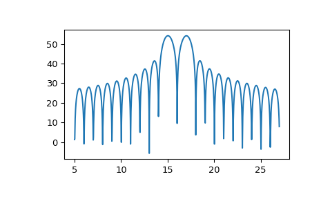
To plot the transform results use something like the following:
import numpy as np from scipy.signal import zoom_fft t = np.linspace(0, 1, 1021) x = np.cos(2np.pi15t) + np.sin(2np.pi17t) f1, f2 = 5, 27 X = zoom_fft(x, [f1, f2], len(x), fs=1021) f = np.linspace(f1, f2, len(x)) import matplotlib.pyplot as plt plt.plot(f, 20*np.log10(np.abs(X))) plt.show()