scipy.special.eval_legendre — SciPy v1.15.2 Manual (original) (raw)

scipy.special.eval_legendre(n, x, out=None) = <ufunc 'eval_legendre'>#

Evaluate Legendre polynomial at a point.

The Legendre polynomials can be defined via the Gauss hypergeometric function \({}_2F_1\) as

\[P_n(x) = {}_2F_1(-n, n + 1; 1; (1 - x)/2).\]

When \(n\) is an integer the result is a polynomial of degree\(n\). See 22.5.49 in [AS] for details.

Parameters:

narray_like

Degree of the polynomial. If not an integer, the result is determined via the relation to the Gauss hypergeometric function.

xarray_like

Points at which to evaluate the Legendre polynomial

outndarray, optional

Optional output array for the function values

Returns:

Pscalar or ndarray

Values of the Legendre polynomial

References

[AS]

Milton Abramowitz and Irene A. Stegun, eds. Handbook of Mathematical Functions with Formulas, Graphs, and Mathematical Tables. New York: Dover, 1972.

Examples

import numpy as np from scipy.special import eval_legendre

Evaluate the zero-order Legendre polynomial at x = 0

eval_legendre(0, 0) 1.0

Evaluate the first-order Legendre polynomial between -1 and 1

X = np.linspace(-1, 1, 5) # Domain of Legendre polynomials eval_legendre(1, X) array([-1. , -0.5, 0. , 0.5, 1. ])

Evaluate Legendre polynomials of order 0 through 4 at x = 0

N = range(0, 5) eval_legendre(N, 0) array([ 1. , 0. , -0.5 , 0. , 0.375])

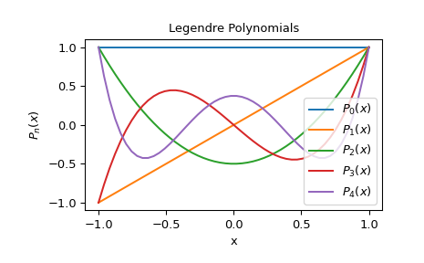
Plot Legendre polynomials of order 0 through 4

X = np.linspace(-1, 1)

import matplotlib.pyplot as plt for n in range(0, 5): ... y = eval_legendre(n, X) ... plt.plot(X, y, label=r'$P_{}(x)$'.format(n))

plt.title("Legendre Polynomials") plt.xlabel("x") plt.ylabel(r'$P_n(x)$') plt.legend(loc='lower right') plt.show()