scipy.special.fdtri — SciPy v1.15.3 Manual (original) (raw)

scipy.special.fdtri(dfn, dfd, p, out=None) = <ufunc 'fdtri'>#

The _p_-th quantile of the F-distribution.

This function is the inverse of the F-distribution CDF, fdtr, returning the x such that fdtr(dfn, dfd, x) = p.

Parameters:

dfnarray_like

First parameter (positive float).

dfdarray_like

Second parameter (positive float).

parray_like

Cumulative probability, in [0, 1].

outndarray, optional

Optional output array for the function values

Returns:

xscalar or ndarray

The quantile corresponding to p.

See also

fdtr

F distribution cumulative distribution function

fdtrc

F distribution survival function

scipy.stats.f

F distribution

Notes

The computation is carried out using the relation to the inverse regularized beta function, \(I^{-1}_x(a, b)\). Let\(z = I^{-1}_p(d_d/2, d_n/2).\) Then,

\[x = \frac{d_d (1 - z)}{d_n z}.\]

If p is such that \(x < 0.5\), the following relation is used instead for improved stability: let\(z' = I^{-1}_{1 - p}(d_n/2, d_d/2).\) Then,

\[x = \frac{d_d z'}{d_n (1 - z')}.\]

Wrapper for the Cephes [1] routine fdtri.

The F distribution is also available as scipy.stats.f. Callingfdtri directly can improve performance compared to the ppfmethod of scipy.stats.f (see last example below).

References

Examples

fdtri represents the inverse of the F distribution CDF which is available as fdtr. Here, we calculate the CDF for df1=1, df2=2at x=3. fdtri then returns 3 given the same values for df1,df2 and the computed CDF value.

import numpy as np from scipy.special import fdtri, fdtr df1, df2 = 1, 2 x = 3 cdf_value = fdtr(df1, df2, x) fdtri(df1, df2, cdf_value) 3.000000000000006

Calculate the function at several points by providing a NumPy array for_x_.

x = np.array([0.1, 0.4, 0.7]) fdtri(1, 2, x) array([0.02020202, 0.38095238, 1.92156863])

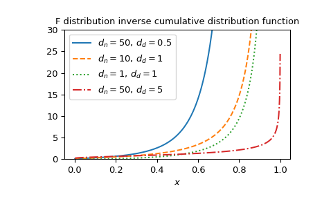
Plot the function for several parameter sets.

import matplotlib.pyplot as plt dfn_parameters = [50, 10, 1, 50] dfd_parameters = [0.5, 1, 1, 5] linestyles = ['solid', 'dashed', 'dotted', 'dashdot'] parameters_list = list(zip(dfn_parameters, dfd_parameters, ... linestyles)) x = np.linspace(0, 1, 1000) fig, ax = plt.subplots() for parameter_set in parameters_list: ... dfn, dfd, style = parameter_set ... fdtri_vals = fdtri(dfn, dfd, x) ... ax.plot(x, fdtri_vals, label=rf"$d_n={dfn},, d_d={dfd}$", ... ls=style) ax.legend() ax.set_xlabel("$x$") title = "F distribution inverse cumulative distribution function" ax.set_title(title) ax.set_ylim(0, 30) plt.show()

The F distribution is also available as scipy.stats.f. Using fdtridirectly can be much faster than calling the ppf method ofscipy.stats.f, especially for small arrays or individual values. To get the same results one must use the following parametrization:stats.f(dfn, dfd).ppf(x)=fdtri(dfn, dfd, x).

from scipy.stats import f dfn, dfd = 1, 2 x = 0.7 fdtri_res = fdtri(dfn, dfd, x) # this will often be faster than below f_dist_res = f(dfn, dfd).ppf(x) f_dist_res == fdtri_res # test that results are equal True