scipy.special.gdtr — SciPy v1.15.3 Manual (original) (raw)

scipy.special.gdtr(a, b, x, out=None) = <ufunc 'gdtr'>#

Gamma distribution cumulative distribution function.

Returns the integral from zero to x of the gamma probability density function,

\[F = \int_0^x \frac{a^b}{\Gamma(b)} t^{b-1} e^{-at}\,dt,\]

where \(\Gamma\) is the gamma function.

Parameters:

aarray_like

The rate parameter of the gamma distribution, sometimes denoted\(\beta\) (float). It is also the reciprocal of the scale parameter \(\theta\).

barray_like

The shape parameter of the gamma distribution, sometimes denoted\(\alpha\) (float).

xarray_like

The quantile (upper limit of integration; float).

outndarray, optional

Optional output array for the function values

Returns:

Fscalar or ndarray

The CDF of the gamma distribution with parameters a and _b_evaluated at x.

Notes

The evaluation is carried out using the relation to the incomplete gamma integral (regularized gamma function).

Wrapper for the Cephes [1] routine gdtr. Calling gdtr directly can improve performance compared to the cdf method of scipy.stats.gamma(see last example below).

References

Examples

Compute the function for a=1, b=2 at x=5.

import numpy as np from scipy.special import gdtr import matplotlib.pyplot as plt gdtr(1., 2., 5.) 0.9595723180054873

Compute the function for a=1 and b=2 at several points by providing a NumPy array for x.

xvalues = np.array([1., 2., 3., 4]) gdtr(1., 1., xvalues) array([0.63212056, 0.86466472, 0.95021293, 0.98168436])

gdtr can evaluate different parameter sets by providing arrays with broadcasting compatible shapes for a, b and x. Here we compute the function for three different a at four positions x and b=3, resulting in a 3x4 array.

a = np.array([[0.5], [1.5], [2.5]]) x = np.array([1., 2., 3., 4]) a.shape, x.shape ((3, 1), (4,))

gdtr(a, 3., x) array([[0.01438768, 0.0803014 , 0.19115317, 0.32332358], [0.19115317, 0.57680992, 0.82642193, 0.9380312 ], [0.45618688, 0.87534798, 0.97974328, 0.9972306 ]])

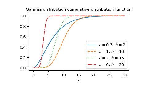
Plot the function for four different parameter sets.

a_parameters = [0.3, 1, 2, 6] b_parameters = [2, 10, 15, 20] linestyles = ['solid', 'dashed', 'dotted', 'dashdot'] parameters_list = list(zip(a_parameters, b_parameters, linestyles)) x = np.linspace(0, 30, 1000) fig, ax = plt.subplots() for parameter_set in parameters_list: ... a, b, style = parameter_set ... gdtr_vals = gdtr(a, b, x) ... ax.plot(x, gdtr_vals, label=fr"$a= {a},, b={b}$", ls=style) ax.legend() ax.set_xlabel("$x$") ax.set_title("Gamma distribution cumulative distribution function") plt.show()

The gamma distribution is also available as scipy.stats.gamma. Usinggdtr directly can be much faster than calling the cdf method ofscipy.stats.gamma, especially for small arrays or individual values. To get the same results one must use the following parametrization:stats.gamma(b, scale=1/a).cdf(x)=gdtr(a, b, x).

from scipy.stats import gamma a = 2. b = 3 x = 1. gdtr_result = gdtr(a, b, x) # this will often be faster than below gamma_dist_result = gamma(b, scale=1/a).cdf(x) gdtr_result == gamma_dist_result # test that results are equal True