scipy.special.nbdtri — SciPy v1.15.3 Manual (original) (raw)
scipy.special.nbdtri(k, n, y, out=None) = <ufunc 'nbdtri'>#
Returns the inverse with respect to the parameter p ofy = nbdtr(k, n, p), the negative binomial cumulative distribution function.
Parameters:
karray_like
The maximum number of allowed failures (nonnegative int).
narray_like
The target number of successes (positive int).
yarray_like
The probability of k or fewer failures before n successes (float).
outndarray, optional
Optional output array for the function results
Returns:
pscalar or ndarray
Probability of success in a single event (float) such that_nbdtr(k, n, p) = y_.
See also
Cumulative distribution function of the negative binomial.
Negative binomial survival function.
negative binomial distribution.
Inverse with respect to k of nbdtr(k, n, p).
Inverse with respect to n of nbdtr(k, n, p).
Negative binomial distribution
Notes
Wrapper for the Cephes [1] routine nbdtri.
The negative binomial distribution is also available asscipy.stats.nbinom. Using nbdtri directly can improve performance compared to the ppf method of scipy.stats.nbinom.
References
Examples
nbdtri is the inverse of nbdtr with respect to p. Up to floating point errors the following holds:nbdtri(k, n, nbdtr(k, n, p))=p.
import numpy as np from scipy.special import nbdtri, nbdtr k, n, y = 5, 10, 0.2 cdf_val = nbdtr(k, n, y) nbdtri(k, n, cdf_val) 0.20000000000000004
Compute the function for k=10 and n=5 at several points by providing a NumPy array or list for y.
y = np.array([0.1, 0.4, 0.8]) nbdtri(3, 5, y) array([0.34462319, 0.51653095, 0.69677416])
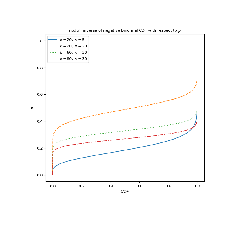
Plot the function for three different parameter sets.
import matplotlib.pyplot as plt n_parameters = [5, 20, 30, 30] k_parameters = [20, 20, 60, 80] linestyles = ['solid', 'dashed', 'dotted', 'dashdot'] parameters_list = list(zip(n_parameters, k_parameters, linestyles)) cdf_vals = np.linspace(0, 1, 1000) fig, ax = plt.subplots(figsize=(8, 8)) for parameter_set in parameters_list: ... n, k, style = parameter_set ... nbdtri_vals = nbdtri(k, n, cdf_vals) ... ax.plot(cdf_vals, nbdtri_vals, label=rf"$k={k},\ n={n}$", ... ls=style) ax.legend() ax.set_ylabel("$p$") ax.set_xlabel("$CDF$") title = "nbdtri: inverse of negative binomial CDF with respect to ppp" ax.set_title(title) plt.show()
nbdtri can evaluate different parameter sets by providing arrays with shapes compatible for broadcasting for k, n and p. Here we compute the function for three different k at four locations p, resulting in a 3x4 array.
k = np.array([[5], [10], [15]]) y = np.array([0.3, 0.5, 0.7, 0.9]) k.shape, y.shape ((3, 1), (4,))
nbdtri(k, 5, y) array([[0.37258157, 0.45169416, 0.53249956, 0.64578407], [0.24588501, 0.30451981, 0.36778453, 0.46397088], [0.18362101, 0.22966758, 0.28054743, 0.36066188]])