order_statistic — SciPy v1.15.2 Manual (original) (raw)

scipy.stats.

scipy.stats.order_statistic(X, /, *, r, n)[source]#

Probability distribution of an order statistic

Returns a random variable that follows the distribution underlying the\(r^{\text{th}}\) order statistic of a sample of \(n\)observations of a random variable \(X\).

Parameters:

XContinuousDistribution

The random variable \(X\)

rarray_like

The (positive integer) rank of the order statistic \(r\)

narray_like

The (positive integer) sample size \(n\)

Returns:

YContinuousDistribution

A random variable that follows the distribution of the prescribed order statistic.

Notes

If we make \(n\) observations of a continuous random variable\(X\) and sort them in increasing order\(X_{(1)}, \dots, X_{(r)}, \dots, X_{(n)}\),\(X_{(r)}\) is known as the \(r^{\text{th}}\) order statistic.

If the PDF, CDF, and CCDF underlying math:X are denoted \(f\),\(F\), and \(F'\), respectively, then the PDF underlying math:X_{(r)} is given by:

\[f_r(x) = \frac{n!}{(r-1)! (n-r)!} f(x) F(x)^{r-1} F'(x)^{n - r}\]

The CDF and other methods of the distribution underlying \(X_{(r)}\)are calculated using the fact that \(X = F^{-1}(U)\), where \(U\) is a standard uniform random variable, and that the order statistics of observations of U follow a beta distribution, \(B(r, n - r + 1)\).

References

Examples

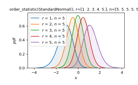
Suppose we are interested in order statistics of samples of size five drawn from the standard normal distribution. Plot the PDF underlying each order statistic and compare with a normalized histogram from simulation.

import numpy as np import matplotlib.pyplot as plt from scipy import stats

X = stats.Normal() data = X.sample(shape=(10000, 5)) sorted = np.sort(data, axis=1) Y = stats.order_statistic(X, r=[1, 2, 3, 4, 5], n=5)

ax = plt.gca() colors = plt.rcParams['axes.prop_cycle'].by_key()['color'] for i in range(5): ... y = sorted[:, i] ... ax.hist(y, density=True, bins=30, alpha=0.1, color=colors[i]) Y.plot(ax=ax) plt.show()