scipy.stats.rel_breitwigner — SciPy v1.15.2 Manual (original) (raw)
scipy.stats.rel_breitwigner = <scipy.stats._continuous_distns.rel_breitwigner_gen object>[source]#
A relativistic Breit-Wigner random variable.
As an instance of the rv_continuous class, rel_breitwigner object inherits from it a collection of generic methods (see below for the full list), and completes them with details specific for this particular distribution.
See also
Cauchy distribution, also known as the Breit-Wigner distribution.
Notes
The probability density function for rel_breitwigner is
\[f(x, \rho) = \frac{k}{(x^2 - \rho^2)^2 + \rho^2}\]
where
\[k = \frac{2\sqrt{2}\rho^2\sqrt{\rho^2 + 1}} {\pi\sqrt{\rho^2 + \rho\sqrt{\rho^2 + 1}}}\]
The relativistic Breit-Wigner distribution is used in high energy physics to model resonances [1]. It gives the uncertainty in the invariant mass,\(M\) [2], of a resonance with characteristic mass \(M_0\) and decay-width \(\Gamma\), where \(M\), \(M_0\) and \(\Gamma\)are expressed in natural units. In SciPy’s parametrization, the shape parameter \(\rho\) is equal to \(M_0/\Gamma\) and takes values in\((0, \infty)\).
Equivalently, the relativistic Breit-Wigner distribution is said to give the uncertainty in the center-of-mass energy \(E_{\text{cm}}\). In natural units, the speed of light \(c\) is equal to 1 and the invariant mass \(M\) is equal to the rest energy \(Mc^2\). In the center-of-mass frame, the rest energy is equal to the total energy [3].
The probability density above is defined in the “standardized” form. To shift and/or scale the distribution use the loc and scale parameters. Specifically, rel_breitwigner.pdf(x, rho, loc, scale) is identically equivalent to rel_breitwigner.pdf(y, rho) / scale withy = (x - loc) / scale. Note that shifting the location of a distribution does not make it a “noncentral” distribution; noncentral generalizations of some distributions are available in separate classes.
\(\rho = M/\Gamma\) and \(\Gamma\) is the scale parameter. For example, if one seeks to model the \(Z^0\) boson with \(M_0 \approx 91.1876 \text{ GeV}\) and \(\Gamma \approx 2.4952\text{ GeV}\) [4] one can set rho=91.1876/2.4952 and scale=2.4952.
To ensure a physically meaningful result when using the fit method, one should set floc=0 to fix the location parameter to 0.
References
[4]
M. Tanabashi et al. (Particle Data Group) Phys. Rev. D 98, 030001 - Published 17 August 2018
Examples
import numpy as np from scipy.stats import rel_breitwigner import matplotlib.pyplot as plt fig, ax = plt.subplots(1, 1)
Calculate the first four moments:
rho = 36.5 mean, var, skew, kurt = rel_breitwigner.stats(rho, moments='mvsk')
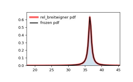
Display the probability density function (pdf):
x = np.linspace(rel_breitwigner.ppf(0.01, rho), ... rel_breitwigner.ppf(0.99, rho), 100) ax.plot(x, rel_breitwigner.pdf(x, rho), ... 'r-', lw=5, alpha=0.6, label='rel_breitwigner pdf')
Alternatively, the distribution object can be called (as a function) to fix the shape, location and scale parameters. This returns a “frozen” RV object holding the given parameters fixed.
Freeze the distribution and display the frozen pdf:
rv = rel_breitwigner(rho) ax.plot(x, rv.pdf(x), 'k-', lw=2, label='frozen pdf')
Check accuracy of cdf and ppf:
vals = rel_breitwigner.ppf([0.001, 0.5, 0.999], rho) np.allclose([0.001, 0.5, 0.999], rel_breitwigner.cdf(vals, rho)) True
Generate random numbers:
r = rel_breitwigner.rvs(rho, size=1000)
And compare the histogram:
ax.hist(r, density=True, bins='auto', histtype='stepfilled', alpha=0.2) ax.set_xlim([x[0], x[-1]]) ax.legend(loc='best', frameon=False) plt.show()
Methods
| rvs(rho, loc=0, scale=1, size=1, random_state=None) | Random variates. |
|---|---|
| pdf(x, rho, loc=0, scale=1) | Probability density function. |
| logpdf(x, rho, loc=0, scale=1) | Log of the probability density function. |
| cdf(x, rho, loc=0, scale=1) | Cumulative distribution function. |
| logcdf(x, rho, loc=0, scale=1) | Log of the cumulative distribution function. |
| sf(x, rho, loc=0, scale=1) | Survival function (also defined as 1 - cdf, but sf is sometimes more accurate). |
| logsf(x, rho, loc=0, scale=1) | Log of the survival function. |
| ppf(q, rho, loc=0, scale=1) | Percent point function (inverse of cdf — percentiles). |
| isf(q, rho, loc=0, scale=1) | Inverse survival function (inverse of sf). |
| moment(order, rho, loc=0, scale=1) | Non-central moment of the specified order. |
| stats(rho, loc=0, scale=1, moments=’mv’) | Mean(‘m’), variance(‘v’), skew(‘s’), and/or kurtosis(‘k’). |
| entropy(rho, loc=0, scale=1) | (Differential) entropy of the RV. |
| fit(data) | Parameter estimates for generic data. See scipy.stats.rv_continuous.fit for detailed documentation of the keyword arguments. |
| expect(func, args=(rho,), loc=0, scale=1, lb=None, ub=None, conditional=False, **kwds) | Expected value of a function (of one argument) with respect to the distribution. |
| median(rho, loc=0, scale=1) | Median of the distribution. |
| mean(rho, loc=0, scale=1) | Mean of the distribution. |
| var(rho, loc=0, scale=1) | Variance of the distribution. |
| std(rho, loc=0, scale=1) | Standard deviation of the distribution. |
| interval(confidence, rho, loc=0, scale=1) | Confidence interval with equal areas around the median. |