scipy.stats.trapezoid — SciPy v1.16.0 Manual (original) (raw)
scipy.stats.trapezoid = <scipy.stats._continuous_distns.trapezoid_gen object>[source]#
A trapezoidal continuous random variable.
As an instance of the rv_continuous class, trapezoid object inherits from it a collection of generic methods (see below for the full list), and completes them with details specific for this particular distribution.
Methods
Notes
The trapezoidal distribution can be represented with an up-sloping line from loc to (loc + c*scale), then constant to (loc + d*scale)and then downsloping from (loc + d*scale) to (loc+scale). This defines the trapezoid base from loc to (loc+scale) and the flat top from c to d proportional to the position along the base with 0 <= c <= d <= 1. When c=d, this is equivalent to triangwith the same values for loc, scale and c. The method of [1] is used for computing moments.
trapezoid takes \(c\) and \(d\) as shape parameters.
The probability density above is defined in the “standardized” form. To shift and/or scale the distribution use the loc and scale parameters. Specifically, trapezoid.pdf(x, c, d, loc, scale) is identically equivalent to trapezoid.pdf(y, c, d) / scale withy = (x - loc) / scale. Note that shifting the location of a distribution does not make it a “noncentral” distribution; noncentral generalizations of some distributions are available in separate classes.
The standard form is in the range [0, 1] with c the mode. The location parameter shifts the start to loc. The scale parameter changes the width from 1 to scale.
References
[1]
Kacker, R.N. and Lawrence, J.F. (2007). Trapezoidal and triangular distributions for Type B evaluation of standard uncertainty. Metrologia 44, 117-127. DOI:10.1088/0026-1394/44/2/003
Examples
import numpy as np from scipy.stats import trapezoid import matplotlib.pyplot as plt fig, ax = plt.subplots(1, 1)
Get the support:
c, d = 0.2, 0.8 lb, ub = trapezoid.support(c, d)
Calculate the first four moments:
mean, var, skew, kurt = trapezoid.stats(c, d, moments='mvsk')
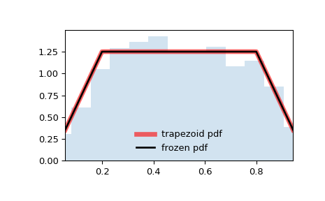
Display the probability density function (pdf):
x = np.linspace(trapezoid.ppf(0.01, c, d), ... trapezoid.ppf(0.99, c, d), 100) ax.plot(x, trapezoid.pdf(x, c, d), ... 'r-', lw=5, alpha=0.6, label='trapezoid pdf')
Alternatively, the distribution object can be called (as a function) to fix the shape, location and scale parameters. This returns a “frozen” RV object holding the given parameters fixed.
Freeze the distribution and display the frozen pdf:
rv = trapezoid(c, d) ax.plot(x, rv.pdf(x), 'k-', lw=2, label='frozen pdf')
Check accuracy of cdf and ppf:
vals = trapezoid.ppf([0.001, 0.5, 0.999], c, d) np.allclose([0.001, 0.5, 0.999], trapezoid.cdf(vals, c, d)) True
Generate random numbers:
r = trapezoid.rvs(c, d, size=1000)
And compare the histogram:
ax.hist(r, density=True, bins='auto', histtype='stepfilled', alpha=0.2) ax.set_xlim([x[0], x[-1]]) ax.legend(loc='best', frameon=False) plt.show()